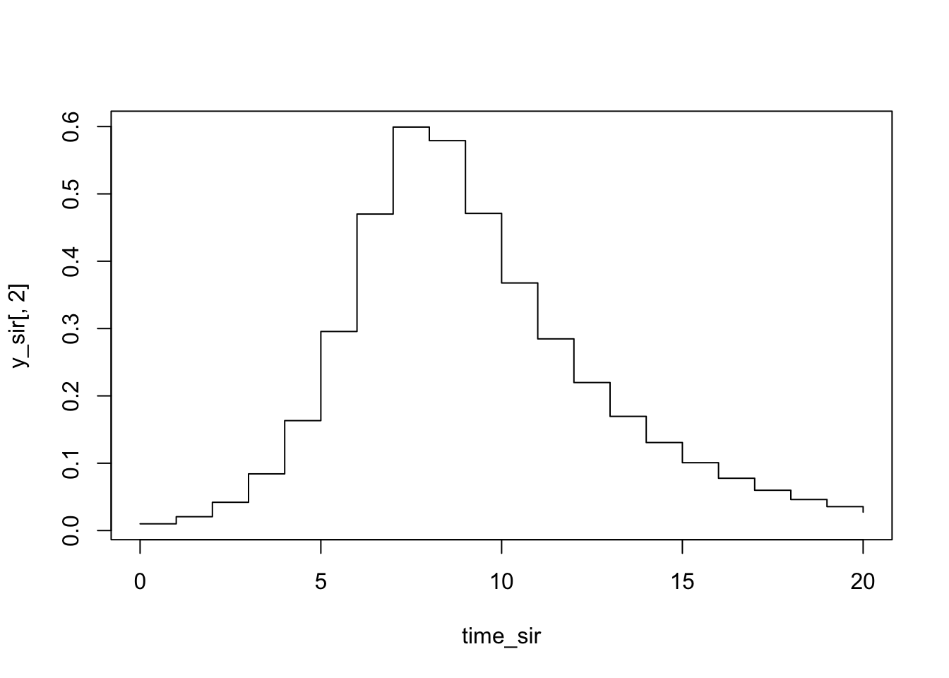
03. Discrete-time deterministic models: Solutions

Practical 1. A simple SIR model

# Times for evaluating the model
time_sir <- seq(0, 20, by = 1)

# Storage for S, I, R at times time_sir
y_sir <- matrix(data = NA,
                nrow = length(time_sir),
                ncol = 3)

# Function to return our update vector with three elements:
update_sir <- function(t, y, parms)
{
    # Get parameter values from parms vector
    beta  <- parms["beta"]
    gamma <- parms["gamma"]
    
    # Get current state variables from y vector
    S <- y[1]
    I <- y[2]
    R <- y[3]

    # Numeric vector with updates to add to S, I, and R respectively
    out <- c(-beta * S * I,
              beta * S * I - gamma * I,
                             gamma * I)

    return (out)
}

# Set parameter values
parms_sir <- c(beta = 1.3, gamma = 0.23)

# Set initial values for time zero
y_sir[1, ] <- c(0.99, 0.01, 0)

# Run each step of the model from the second time step onward
for (i in 2:nrow(y_sir))
{
    # Assign new value to y_sir[i, ] using the update_sir function
    y_sir[i, ] <- y_sir[i - 1, ] +
        update_sir(time_sir[i],
                   y_sir[i - 1, ],
                   parms_sir)
}

# Plot the number of infectious individuals over time
# type = "s" makes a "stair-step" line plot suitable for difference equations
plot(x = time_sir, y = y_sir[, 2], type = "s")

Questions 1-6 ask:

At approximately what time does the peak in infectious population occur and what proportion of the population is infectious? and
Approximately what proportion of the population gets infected?

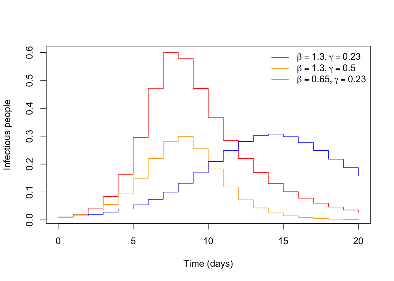
for three different sets of beta (transmission rate) and gamma (recovery rate) in the model. The solutions are summarized in the table and figure below:

Parameters	Peak in infectious population	Total proportion infected
`beta = 1.3, gamma = 0.23`	(1) t = 7, I = 0.60	(2) 0.9997
`beta = 1.3, gamma = 0.5`	(3) t = 8, I = 0.30	(4) 0.943
`beta = 0.65, gamma = 0.23`	(5) t = 14, I = 0.31	(6) 0.943

When we start with $β = 1.3, γ = 0.23$ the peak occurs on day 7 with 60% of the population infectious. Almost everyone in the population is infected by the end of the simulation.

When we increase gamma from $γ = 0.23$ to $γ = 0.5$ , this increase in the recovery rate corresponds to a shorter infectious period (2 days instead of 4.35 days). This means people spend less time in the $I$ compartment, which decreases the reproduction number by around $1 / 2$ , and so the peak proportion of the population who are infectious is smaller (by around $1 / 2$ ). But since the generation interval is also shorter by around $1 / 2$ , the peak doesn’t happen substantially later.

When instead we decrease beta from $β = 1.3$ to $β = 0.65$ , this decrease in the transmission rate reduces the reproduction number, but does not change the generation interval. The peak proportion of the population who are infectious is smaller relative to when $β = 1.3, γ = 0.23$ . This time, the peak is also shifted later, because the lower reproduction number is not “compensated” in this regard by a shorter generation interval.

For questions (4) and (6), the reproduction number is lower by around the same amount relative to question (2), so the total proportion infected is lower by a similar amount in both (4) and (6).

Practical 2. Extending the SIR model

Incorporating births and deaths

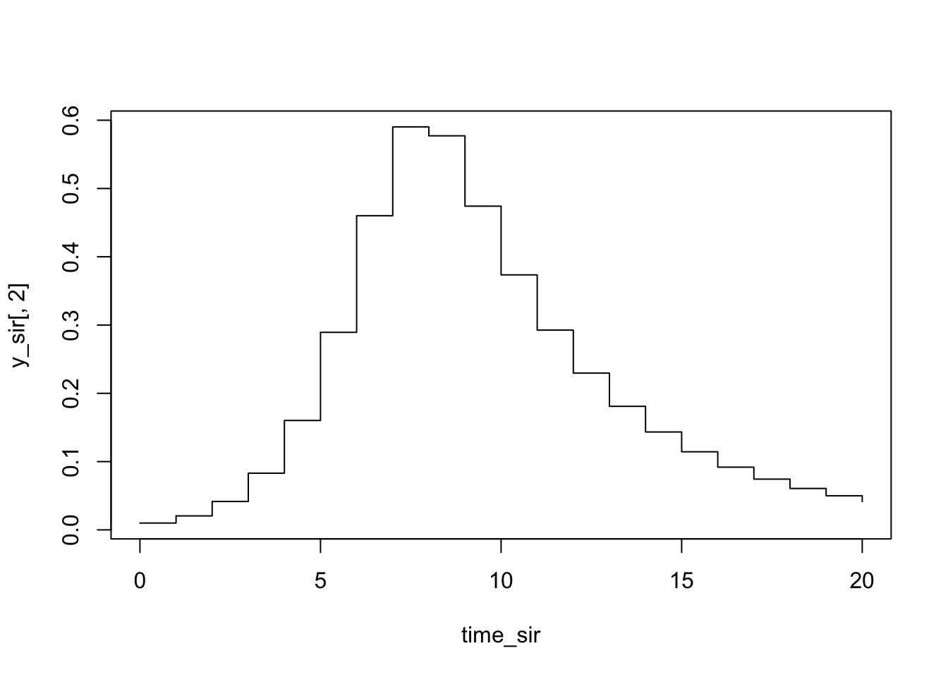
# Times for evaluating the model
time_sir <- seq(0, 20, by = 1)

# Storage for S, I, R at times time_sir
y_sir <- matrix(data = NA,
                nrow = length(time_sir),
                ncol = 3)

# Function to return our update vector with three elements:
update_sir <- function(t, y, parms)
{
    # Get parameter values from parms vector
    beta  <- parms["beta"]
    gamma <- parms["gamma"]
    delta <- parms["delta"] ## NEW: delta parameter
    
    # Get current state variables from y vector
    S <- y[1]
    I <- y[2]
    R <- y[3]
    N <- S + I + R ## NEW: calculation of N

    # Numeric vector with updates to add to S, I, and R respectively
    ## NEW: transitions for birth and death with parameter delta
    out <- c(-S * delta - beta * S * I + N * delta,
             -I * delta + beta * S * I - gamma * I,
             -R * delta                + gamma * I)

    return (out)
}

# Set parameter values
## NEW: parameter delta
parms_sir <- c(beta = 1.3, gamma = 0.23, delta = 0.01)

# Set initial values for time zero
y_sir[1, ] <- c(0.99, 0.01, 0)

# Run each step of the model from the second time step onward
for (i in 2:nrow(y_sir))
{
    # Assign new value to y_sir[i, ] using the update_sir function
    y_sir[i, ] <- y_sir[i - 1, ] +
        update_sir(time_sir[i],
                   y_sir[i - 1, ],
                   parms_sir)
}

# Plot the number of infectious individuals over time
# type = "s" makes a "stair-step" line plot suitable for difference equations
plot(x = time_sir, y = y_sir[, 2], type = "s")

Visualising for the whole population

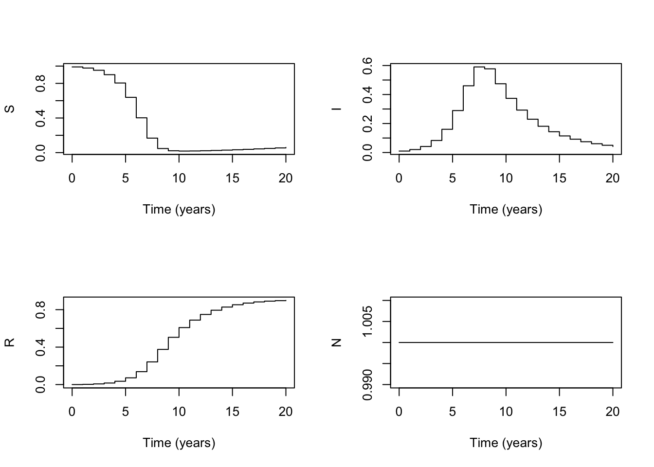
Calculate $N (t) = S (t) + I (t) + R (t)$ the total number of individuals.

Make a plot of $S (t)$ , $I (t)$ , $R (t)$ and $N (t)$ . Your function $N (t)$ should be constant at 1 for all values of $t$ . If this is not the case, ensure the model contains births of new S proportional to N, and deaths of each of S, I, and R.

Answer. Here is one possible method:

# Add total population N(t) to y_sir matrix
y_sir <- cbind(y_sir, rowSums(y_sir))

# Plot each model component
par(mfrow = c(2, 2))
components = c("S", "I", "R", "N")

for (i in 1:ncol(y_sir)) {
    plot(y_sir[, i] ~ time_sir, type = "s", xlab = "Time (years)", ylab = components[i])
}

par(mfrow = c(1, 1))

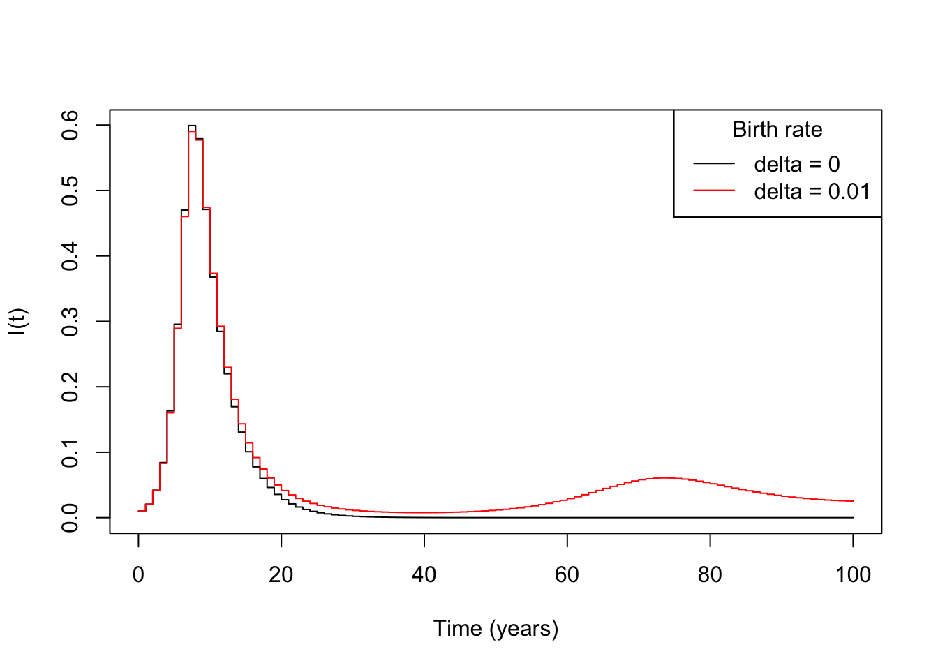
Change the code so the model runs for 100 time steps instead of 20. Compare the number of infectious people over time when delta = 0 (no births and deaths, as before) versus when delta = 0.01. What explains the difference?

Answer. When the birth rate is 0.01, we eventually see a second outbreak occur around year 50. This is because new susceptibles enter the population via birth, which eventually furnishes enough susceptibles to make the effective reproduction number $R_{t} > 1$ and allow a new outbreak to occur.

Here is one way of plotting infectious individuals over time for delta = 0 versus delta = 0.01, assuming that the solution y_sir for delta = 0 is stored in the new variable y_sir_00, and y_sir for delta = 0.01 is stored in the new variable y_sir_01:

plot(time_sir, y_sir_00[, 2], col = "black", type = "s", xlab = "Time (years)", ylab = "I(t)")
lines(time_sir, y_sir_01[, 2], col = "red", type = "s", xlab = "Time (years)")
legend("topright", c("delta = 0", "delta = 0.01"), col = c("black", "red"), lty = 1, title = "Birth rate")

Describe the parameters of the model, what they represent, and whether the assumptions they represent are realistic.

Answer:

The transmission rate beta represents the rate at which an individual makes “effective contact” with another individual, where effective contact results in a new infection if the contacted individual is infectious and the contacting individual is susceptible.

The recovery rate gamma represents the recovery rate, such that 1/gamma is the infectious period.

The birth rate delta captures the rate of new births and also the rate of deaths.

There’s an implicit assumption in the model that transmission is not passed to newborns, i.e., only susceptibles are born. This is likely a reasonable assumption to make for many diseases.

As we are dealing with proportions of the total population, it’s reasonable to keep N(t) constant, but the birth and death rates may not be reasonable.

Additionally, we assume that the birth rate is proportional to the entire population, rather than restricting our attention to individuals of reproductive age. We also assume that the disease itself does not cause a loss of life expectancy.

Click here to return to the practical.