04. Ordinary differential equations (ODEs): SEIRV model

Practical 1: Susceptible-Exposed-Infectious-Recovered-Vaccinated model implementation

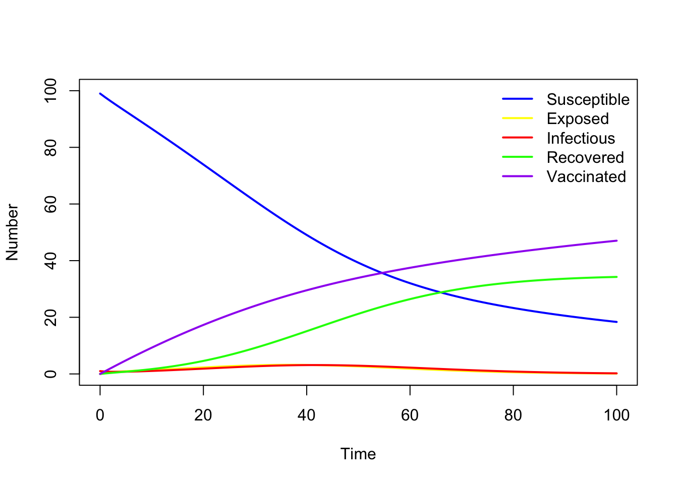
library(deSolve) # For solving systems of ODEs

# Define model function
SEIRV_model <- function(times, state, parms)
{
    # Get variables
    S <- state["S"]
    E <- state["E"]
    I <- state["I"]
    R <- state["R"]
    V <- state["V"]
    N <- S + E + I + R + V
    # Get parameters
    beta <- parms["beta"]
    delta <- parms["delta"]
    gamma <- parms["gamma"]
    v <- parms["v"]
    # Define differential equations
    dS <- -(beta * I / N) * S - v * S
    dE <- (beta * I / N) * S - delta * E
    dI <- delta * E - gamma * I
    dR <- gamma * I
    dV <- v * S
    res <- list(c(dS, dE, dI, dR, dV))
    return (res)
}

# Define parameter values
parms <- c(beta = 0.4, delta = 0.2, gamma = 0.2, v = 0.01)

# Define time to solve equations
times <- seq(from = 0, to = 100, by = 1)

# Define initial conditions
N <- 100
E_0 <- 0
I_0 <- 1
R_0 <- 0
V_0 <- 0
S_0 <- N - E_0 - I_0 - R_0 - V_0
y <- c(S = S_0, E = E_0, I = I_0, R = R_0, V = V_0)

# Solve equations
output_raw <- ode(y = y, times = times, func = SEIRV_model, parms = parms)

# Convert matrix to data frame for easier manipulation
output <- as.data.frame(output_raw)

# Plot model output
plot(output$time, output$S, type = "l", col = "blue", lwd = 2, ylim = c(0, N),
      xlab = "Time", ylab = "Number")
lines(output$time, output$E, lwd = 2, col = "yellow", type = "l")
lines(output$time, output$I, lwd = 2, col = "red", type = "l")
lines(output$time, output$R, lwd = 2, col = "green", type = "l")
lines(output$time, output$V, lwd = 2, col = "purple", type = "l")
legend("topright", legend = c("Susceptible", "Exposed", "Infectious", "Recovered", "Vaccinated"),
       col = c("blue", "yellow", "red", "green", "purple"), lwd = 2, bty = "n")