04. Ordinary differential equations (ODEs): SI model

Practical 1: Susceptible-Infectious model implementation

Step-by-step

We will be using the deSolve package for this, so first we need to load the package.

library(deSolve)

If the deSolve package is not installed, first install it using:

install.packages("deSolve")

and then re-run the library(deSolve) line.

Now, we need to put together our initial conditions as a named numeric vector. The names in the vector should correspond to the names of each compartment in our ODE system, i.e. S and I.

y <- c(S = 99, I = 1)

This gives us 99 susceptibles and one infectious individual. Alternatively we can define S in terms of the total population size and the number of initially infectious people:

N <- 100
I_0 <- 1
S_0 <- N - I_0
y <- c(S = S_0, I = I_0)

We also need to define which times we want the solution to be evaluated at. For this practical we are solving from 0 to 50 days in steps of 1 day:

times <- seq(from = 0, to = 50, by = 1)

Now we should define the parameters. There is just one parameter, the transmission rate beta:

parms <- c(beta = 0.4)

Now let’s code up the (ordinary differential) equations themselves in an R function:

SI_model <- function(times, state, parms)
{
    # Get variables
    S <- state["S"]
    I <- state["I"]
    N <- S + I
    # Get parameters
    beta <- parms["beta"]
    # Define differential equations
    dS <- -(beta * I / N) * S
    dI <- (beta * I / N) * S
    res <- list(c(dS, dI))
    return (res)
}

Make sure you understand what is happening in the function above before you continue.

Having assembled all the “ingredients”, we can now solve the ODE model and plot it:

# Solve equations
output_raw <- ode(y = y, times = times, func = SI_model, parms = parms)

# Convert matrix to data frame for easier manipulation
output <- as.data.frame(output_raw)

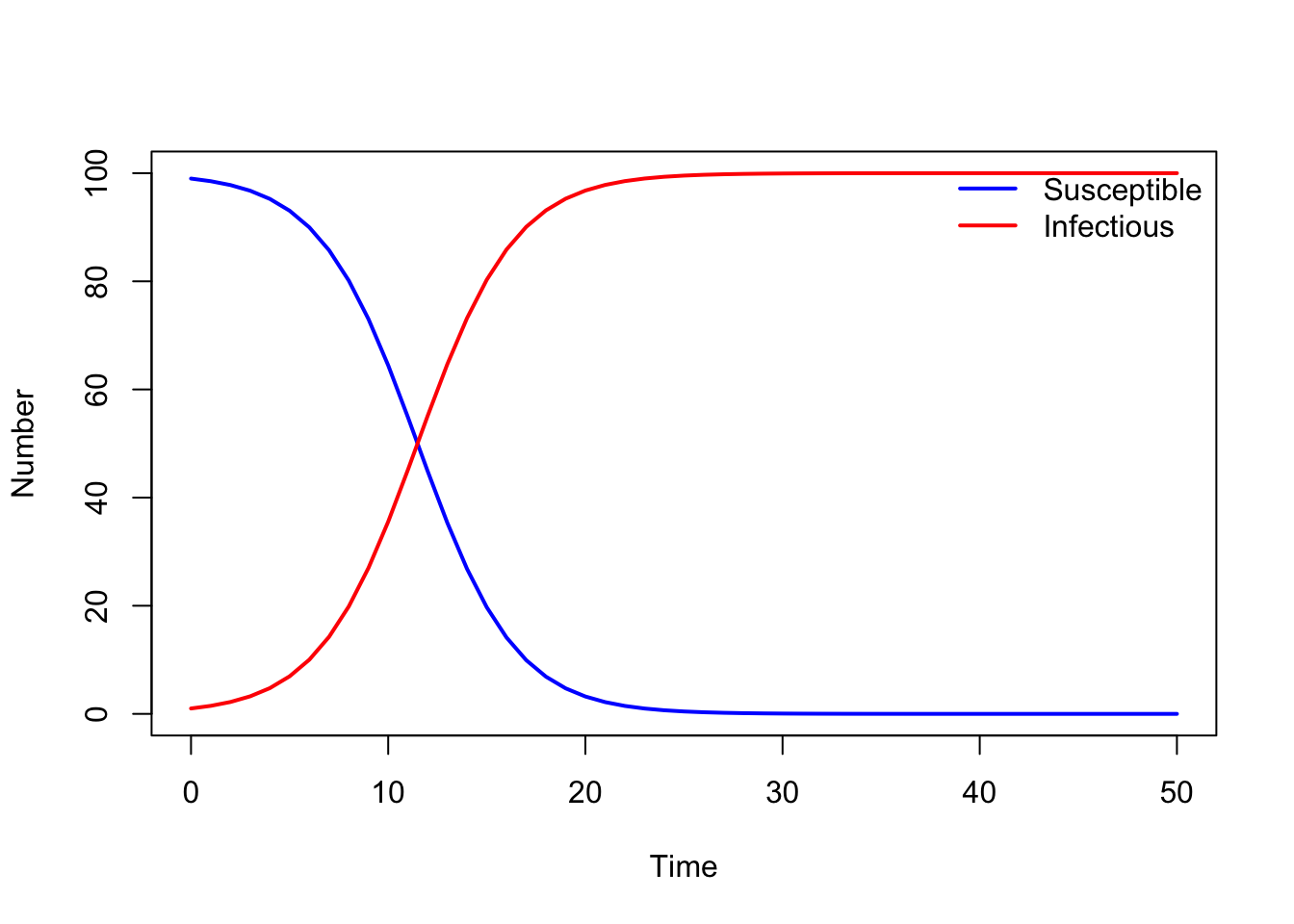
# Plot model output
plot(output$time, output$S, type = "l", col = "blue", lwd = 2, ylim = c(0, N),
      xlab = "Time", ylab = "Number")
lines(output$time, output$I, lwd = 2, col = "red", type = "l")
legend("topright", legend = c("Susceptible", "Infectious"),
       col = c("blue", "red"), lwd = 2, bty = "n")

All together

Bringing all the above pieces together looks something like the following. Note that we have defined the SI model function at the top and the parms, times, and y vectors below so that it is easier to change the parameters or initial conditions and re-run the model without having to scroll up past the model function.

library(deSolve) # For solving systems of ODEs

# Define model function
SI_model <- function(times, state, parms)
{
    # Get variables
    S <- state["S"]
    I <- state["I"]
    N <- S + I
    # Get parameters
    beta <- parms["beta"]
    # Define differential equations
    dS <- -(beta * I / N) * S
    dI <- (beta * I / N) * S
    res <- list(c(dS, dI))
    return (res)
}

# Define parameter values
parms <- c(beta = 0.4)

# Define time to solve equations
times <- seq(from = 0, to = 50, by = 1)

# Define initial conditions
N <- 100
I_0 <- 1
S_0 <- N - I_0
y <- c(S = S_0, I = I_0)

# Solve equations
output_raw <- ode(y = y, times = times, func = SI_model, parms = parms)

# Convert matrix to data frame for easier manipulation
output <- as.data.frame(output_raw)

# Plot model output
plot(output$time, output$S, type = "l", col = "blue", lwd = 2, ylim = c(0, N),
      xlab = "Time", ylab = "Number")
lines(output$time, output$I, lwd = 2, col = "red", type = "l")
legend("topright", legend = c("Susceptible", "Infectious"),
       col = c("blue", "red"), lwd = 2, bty = "n")