05b. Using a contact matrix

This is a short guide to how you might use a contact matrix in a model. This uses the socialmixr package to generate a contact matrix from POLYMOD data for the UK, but you can also define your own contact matrices.

First step is to load in the required packages.

# Load in required packages, deSolve and socialmixr
# If either package is not installed, install using the install.packages() function
library(deSolve)
library(socialmixr)

We now use socialmixr’s contact_matrix function to build a contact matrix from POLYMOD data for the UK. The age.limits argument below specifies that we will consider 10-year age bands, from 0-9 up to 60-69 and finally 70+.

We then extract the contact matrix itself into mat, and gather some info on the number of groups and their names.

polymod_data <- contact_matrix(polymod, countries = "United Kingdom", 
    age.limits = seq(0, 70, by = 10))

Removing participants that have contacts without age information. To change this behaviour, set the 'missing.contact.age' option

mat <- polymod_data$matrix
n_groups <- nrow(mat)
group_names <- rownames(mat)

For more information on socialmixr, try consulting the “socialmixr” vignette by running: vignette("socialmixr", package = "socialmixr").

Let’s take a look at what we have just created:

print(mat)

         contact.age.group
age.group    [0,10)   [10,20)   [20,30)   [30,40)  [40,50)   [50,60)   [60,70)
  [0,10)  5.1522843 1.2487310 1.0964467 2.0203046 1.203046 0.6091371 0.3604061
  [10,20) 1.2318841 8.0628019 1.1739130 1.7294686 1.710145 0.7004831 0.3719807
  [20,30) 1.2711864 1.4406780 3.6016949 1.8898305 1.754237 1.1016949 0.4661017
  [30,40) 1.9384615 1.1230769 1.5153846 2.7615385 1.730769 1.2076923 0.6153846
  [40,50) 0.7863248 1.8547009 1.6153846 2.1794872 2.897436 1.3504274 0.6837607
  [50,60) 0.5583333 0.8916667 1.6333333 1.5500000 1.483333 1.8583333 0.8166667
  [60,70) 0.7096774 0.5913978 1.1720430 1.7204301 1.505376 1.4301075 1.1720430
  70+     0.2758621 1.0000000 0.6896552 0.4482759 1.413793 0.9310345 1.2068966
         contact.age.group
age.group       70+
  [0,10)  0.1421320
  [10,20) 0.1545894
  [20,30) 0.2033898
  [30,40) 0.2923077
  [40,50) 0.5982906
  [50,60) 0.6333333
  [60,70) 0.5483871
  70+     1.3448276

print(n_groups)

[1] 8

print(group_names)

[1] "[0,10)"  "[10,20)" "[20,30)" "[30,40)" "[40,50)" "[50,60)" "[60,70)"
[8] "70+"    

Note the usual pattern with a higher number of contacts along the diagonal. Base R’s matrix plotting functions are a bit tricky, but the lattice package has a relatively easy to use function:

lattice::levelplot(mat)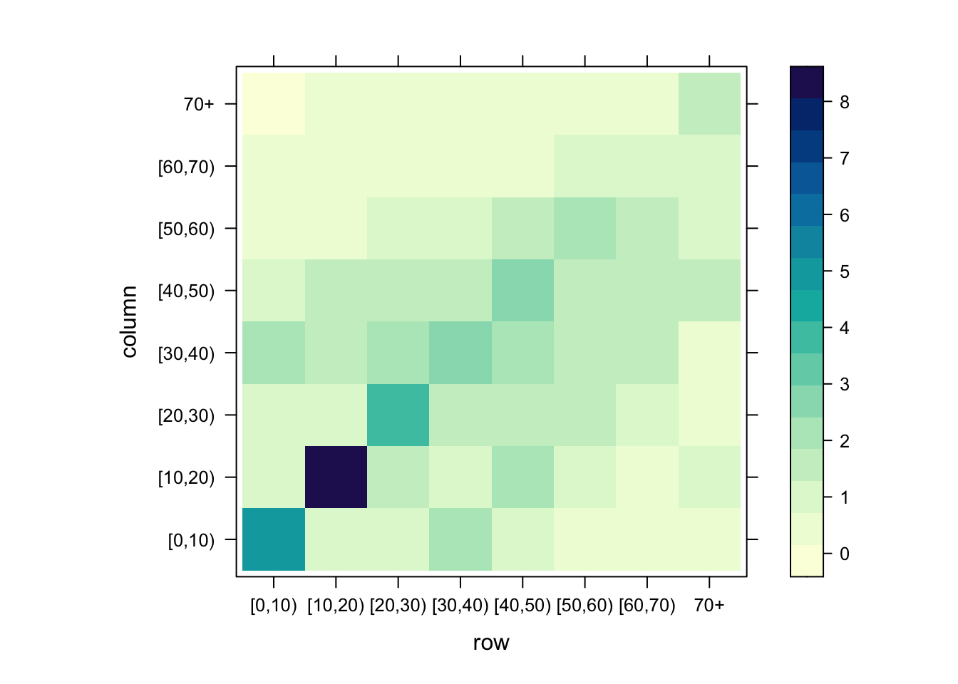

Now let’s start bringing together our model function, initial state, parameters, and times, as normal for an ODE model.

First, the model function:

# Define model function 
SIR_conmat_model <- function(times, state, parms)
{
    # Get variables
    S <- state[1:n_groups]
    I <- state[(n_groups + 1):(2 * n_groups)]
    R <- state[(2 * n_groups + 1):(3 * n_groups)]
    N <- S + I + R
    # Extract parameters
    p <- parms[["p"]]
    cm <- parms[["cm"]]
    gamma <- parms[["gamma"]]
    # Build force of infection
    lambda <- (p * cm %*% (I/N))[,1]
    # Define differential equations
    dS <- -lambda * S
    dI <- lambda * S - gamma * I
    dR <- gamma * I
    res <- list(c(dS, dI, dR))
    return (res)
}

There’s a lot to unpack here, so let’s go step by step.

First, our state vector needs to have n_groups versions of the S compartment, n_groups versions of the I compartment, and n_groups versions of the R compartment. Within the vector, we’ll lay it out in this order: \((S_1, S_2, ..., S_n, I_1, I_2, ..., I_n, R_1, R_2, ..., R_n)\). So, in the lines

    # Get variables
    S <- state[1:n_groups]
    I <- state[(n_groups + 1):(2 * n_groups)]
    R <- state[(2 * n_groups + 1):(3 * n_groups)]
    N <- S + I + R

we’re extracting S, I, and R each as vectors holding n_groups numbers each. Then we’re defining N as the sum of those vectors; it will also hold n_groups numbers, the first one corresponding to the 0-9 age group, the second one corresponding to the 10-19 age group, and so on.

Next we extract parameters:

    # Extract parameters
    p <- parms[["p"]]
    cm <- parms[["cm"]]
    gamma <- parms[["gamma"]]

Notice here we are using double brackets [[ instead of single brackets [[ like we normally do. This is because cm will be our contact matrix, and you can’t really store a matrix inside a vector. You can store it in a list though, which takes double brackets to extract elements.

Now we calculate our force of infection.

    # Build force of infection
    lambda <- (p * cm %*% (I/N))[,1]

This is a bit cryptic, so let’s break it down. What we are doing here is calculating \(\lambda_i = \sum_j c_{ij} I_j/N_j\), for all \(i\). One way of doing this would be with a for loop:

    lambda = rep(0, n_groups)
    for (i in 1:n_groups) {
        lambda[i] <- sum(p * cm[i, ] * I/N)
    }

The line lambda <- (p * cm %*% (I/N))[,1] is equivalent to this, and uses matrix multiplication %*% to achieve what it’s doing. This will run a bit faster in R than the for loop, but either way of calculating the force of infection, lambda (\(\lambda\)), is probably fine.

Finally we define and return the differential equations:

    # Define differential equations
    dS <- -lambda * S
    dI <- lambda * S - gamma * I
    dR <- gamma * I
    res <- list(c(dS, dI, dR))
    return (res)

Remember, S, I, and R are vectors, so dS, dI, and dR are also vectors with length n_groups. The line res <- list(c(dS, dI, dR)) sticks them all together into a vector with n_groups\(\,\times 3\) elements. Then this gets returned.

OK, that’s the end of the model function. Carrying on, we set up the parameters and times (remember, parms will be a list this time instead of a vector):

# Define parameters  
parms <- list(p = 0.05, cm = mat, gamma = 0.2) # NOT c(p = 0.05, cm = mat, gamma = 0.2) !

# Define time to run model
times <- seq(from = 0, to = 50, by = 1)

And define our initial conditions:

# Define initial conditions
N0 <- seq(1000, 650, length.out = n_groups)
I0 <- rep(1, n_groups)
S0 <- N0 - I0
R0 <- rep(0, n_groups)
names(S0) <- paste0("S", 1:n_groups)
names(I0) <- paste0("I", 1:n_groups)
names(R0) <- paste0("R", 1:n_groups)
state <- c(S0, I0, R0)

Note that this sets up the population size so there are 1000 0-9 year olds, 650 70+ year olds, and intermediate numbers in between. Let’s look at our initial state to make sure it’s correct:

print(state)

 S1  S2  S3  S4  S5  S6  S7  S8  I1  I2  I3  I4  I5  I6  I7  I8  R1  R2  R3  R4 
999 949 899 849 799 749 699 649   1   1   1   1   1   1   1   1   0   0   0   0 
 R5  R6  R7  R8 
  0   0   0   0 

Looks good.

Now all we need to do is solve the ODE system and plot it as before:

# Solve equations
output_raw <- ode(y = state, 
                  times = times, 
                  func = SIR_conmat_model, 
                  parms = parms)

# Convert to data frame for easy extraction of columns
output <- as.data.frame(output_raw)

# Plot output
par(mfrow = c(1, 1))
matplot(output$time, output[, 2:ncol(output)], type = "l", xlab = "Time (years)", ylab = "Number of people")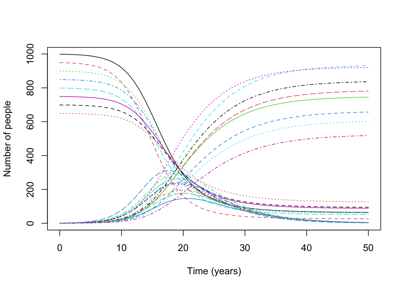

We use matplot here to quickly plot a large number of different lines, each stored in a different column of a matrix. Cool plot, but not so easy to see what’s going on, so let’s split it out by S versus I versus R:

# Make a 2x2 grid
par(mfrow = c(2, 2))
# Plot S, I, R on separate plots
matplot(output$time, output[, (0 * n_groups + 2):(1 * n_groups + 1)], type = "l", 
    xlab = "Time (years)", ylab = "Susceptible", col = rainbow(n_groups), lty = 1)
matplot(output$time, output[, (1 * n_groups + 2):(2 * n_groups + 1)], type = "l", 
    xlab = "Time (years)", ylab = "Infectious", col = rainbow(n_groups), lty = 1)
matplot(output$time, output[, (2 * n_groups + 2):(3 * n_groups + 1)], type = "l", 
    xlab = "Time (years)", ylab = "Recovered", col = rainbow(n_groups), lty = 1)
# Put a legend in the bottom right of the grid
plot.new()
legend("center", legend = rownames(mat), col = rainbow(n_groups), lty = 1)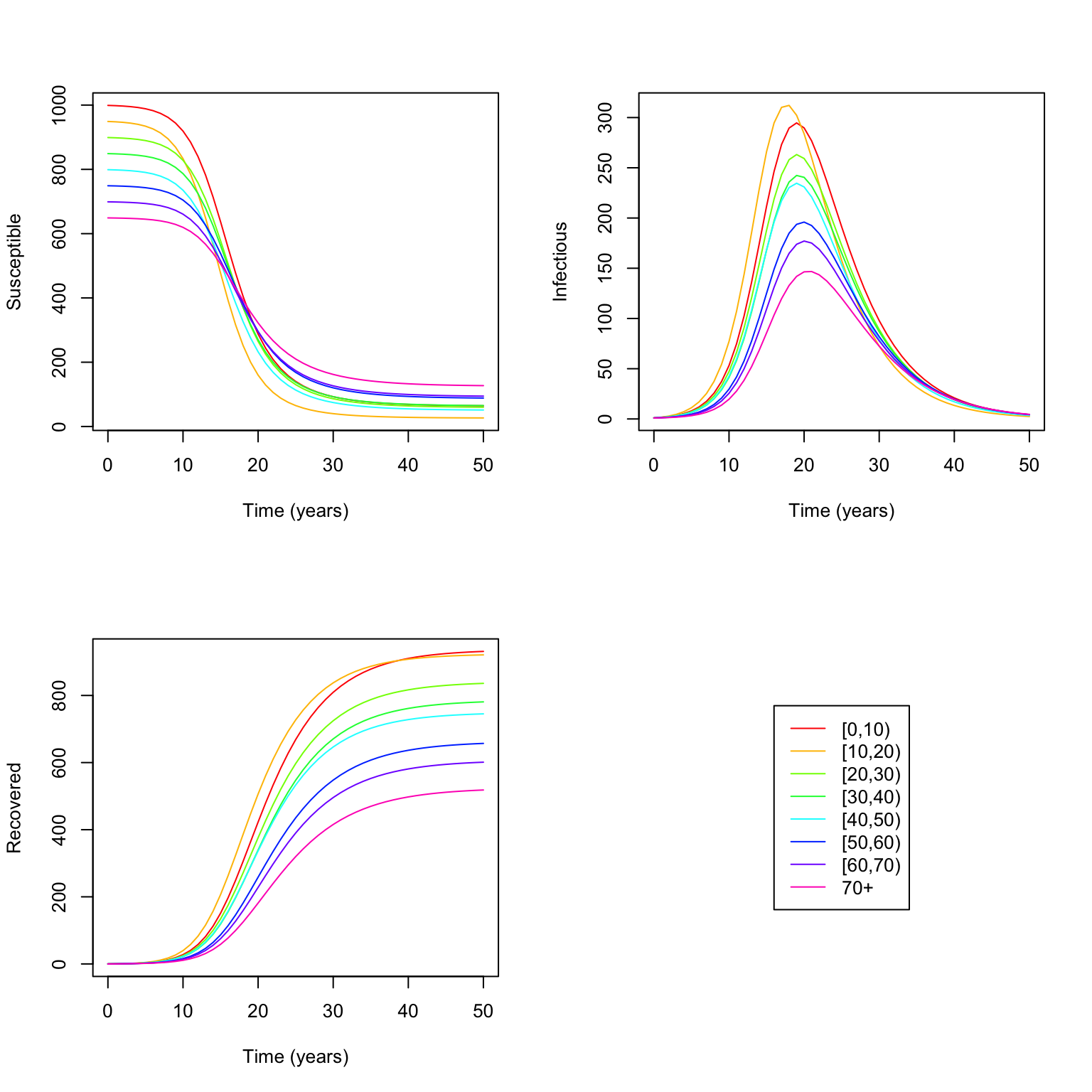

# Put plot grid back to 1x1
par(mfrow = c(1, 1))