First, let’s run an ODE model. Download and open up the SIRmodel.R
(a) Which functions are in here?
Answer: solveODE() and SIR_model()
(b) What are the arguments of the first function?
Answer: (1) the parameter values lists, (2) Argument to plot everything, (3) number of row to plot (4) number of cols to plot
(c) What is the output of the first function?
Answer: maximum prevalence through the epidemic
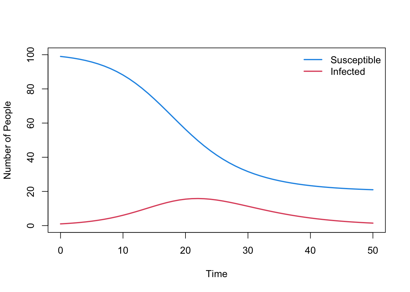
# First let's clear our workspace, remove plots and load the libraries we needrm(list=ls())# dev.off()library(deSolve)library(ggplot2)# Let's read in these functions so we have them to handsource("code/SIRmodel.R")# Let's choose a beta value of 0.4 and a gamma value of 0.2max.prevalence <-solveODE(parameters <-c(beta =0.4, gamma =0.2))
Warning in par(new = TRUE): calling par(new=TRUE) with no plot
print(max.prevalence)
[1] 15.84403
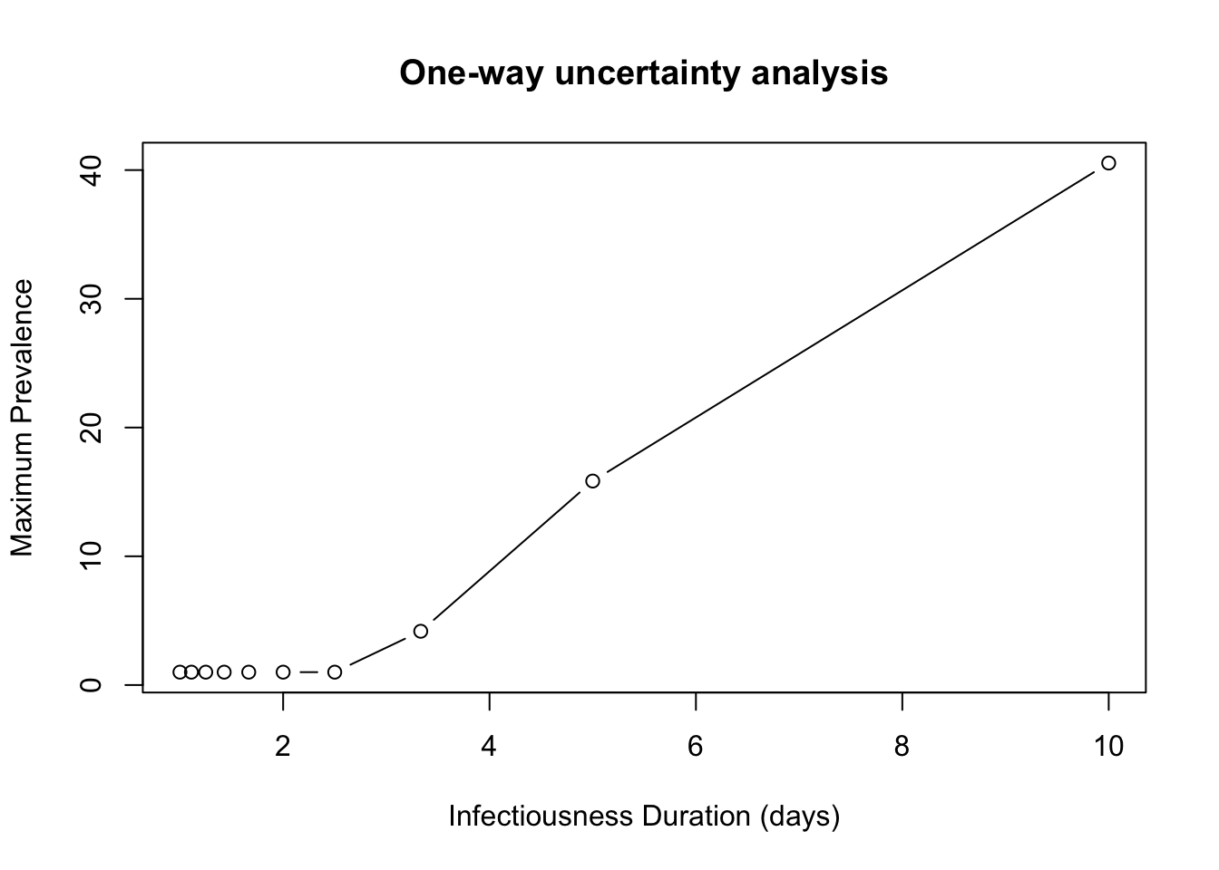
# Now let's look at the effect of the maximum prevalence of the epidemic across # gamma = 0.1 -1.0 (increment on 0.1)gamma.vec <-seq(0.1, 1.0, by =0.1)# initialise max/prevalence containermax.prevalence <-vector()# Add in a loop to make this happenfor (gamma.val in gamma.vec){ mp =solveODE(parameters =c(beta =0.4, gamma = gamma.val),plot.all.results =FALSE) max.prevalence =c(max.prevalence, mp)}
Now we have our max.prevalence, we need to plot this against our infectiousness duration - plot max.prevalence as a function of the infectious duration.
# Now try to increase the resolution of gamma to get a better idea of the # relationship but remember to clear max.prevalence first!# You could try and replace gamma.vec = seq(0.1, 1.0, by = 0.1) withinf.duration =1:10gamma.vec =1/inf.duration
(d) Describe in words the qualitative relationship
Answer: There is no epidemic until the infectiousness duration is > 2 days (R0 > 1) after that there is a linear increase in the maximum prevalence until gamma = 6, then there is a diminishing increase in the maximum prevalence.
(2) Monte Carlo Sampling
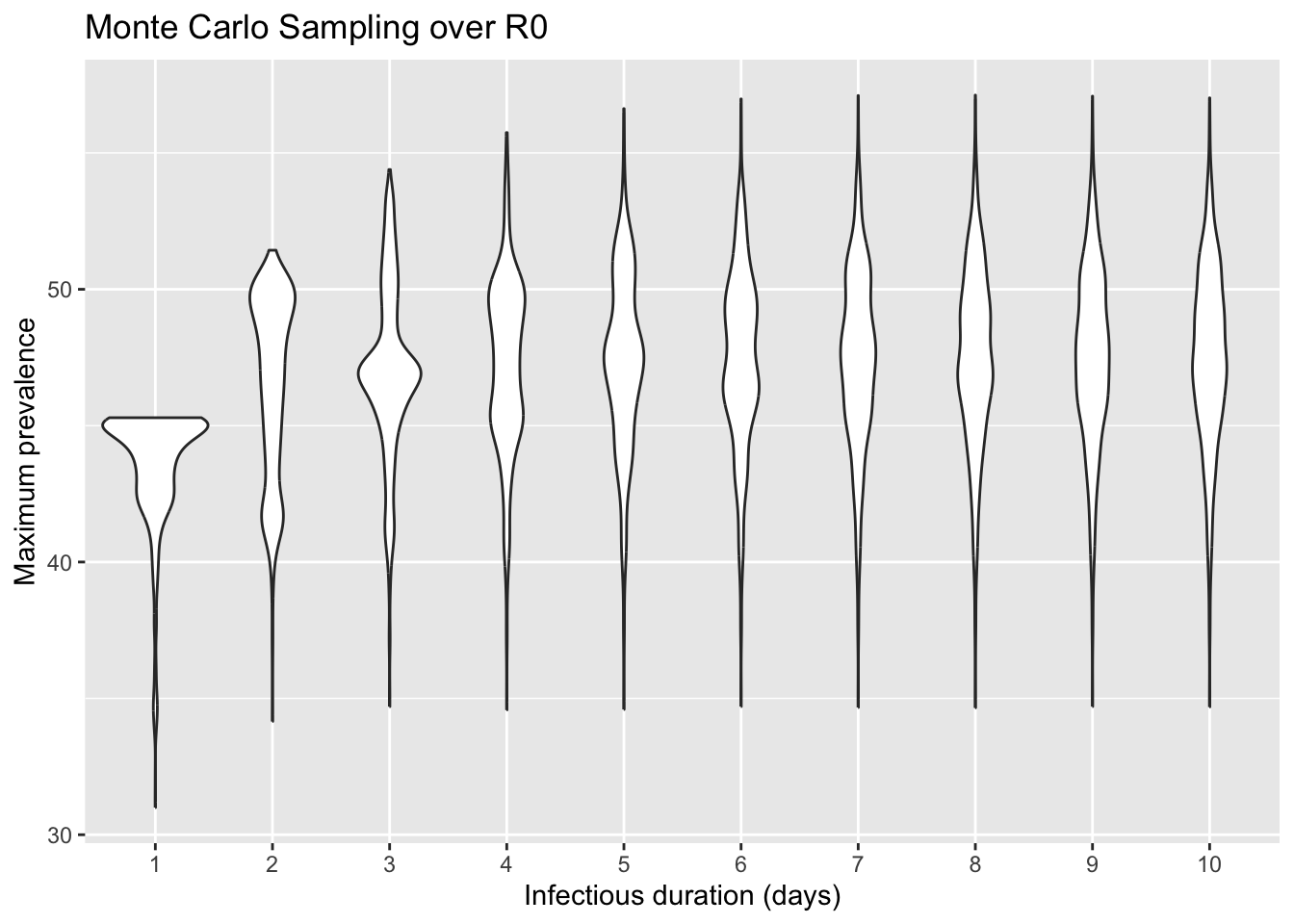
Now suppose that we have a previous epidemiological study that suggested that R0 has a mean value of 5, but uncertainty within the range of [-1, +1]. However, we still don’t know whether the infectiousness period is 1 day or 10 days. We will now use the functions in SIRmodel_R0.R to make a similar plot as above, but this time, incorporate the uncertainty of R0 for each discrete value of gamma. We’re going to first use a direct Monte Carlo Sampling method.
# Read in our set of functions in SIRmodel_R0.Rsource("code/SIRmodel_R0.R")# First, let's set a fixed seed for the random number generator# this will allow us to run the code again and retrieve the same 'simulation'set.seed(2019)# Now, draw R0 1,000 times from a suitable distribution (e.g. normal)r0.all =rnorm(1000, 5, 0.5)size.df =length(r0.all) *length(gamma.vec)# initialise max.prevalence again, this time it needs to be a dataframe # or a matrixmax.prevalence =data.frame(r0.value =vector(mode ="numeric", length = size.df),gamma =vector(mode ="numeric", length = size.df),max.prev =vector(mode ="numeric", length = size.df))index =0# create a loop over each of these R0 values in turnfor (r0.val in r0.all){# create a loop over each of these Gamma values in turnfor (gamma.val in gamma.vec){ index = index +1 mp =solveODE_2(parameters =c(R0 = r0.val, gamma = gamma.val)) max.prevalence[index, "r0.value"] = r0.val max.prevalence[index, "gamma"] = gamma.val max.prevalence[index, "max.prev"] = mp }}# Take a look at max.prevalence by using the 'head() functionhead(max.prevalence)
Answer: using ‘wide’ formatting – see the ggplot pre-course material
# Now plot this output using the R function MCplot() in SIRmodel_R0.RMCplot(max.prevalence)
Warning: Removed 10 rows containing non-finite outside the scale range
(`stat_ydensity()`).
(f) What conclusions can you draw from the plot?
Answer: Increasing the rate of recovery reduces the max prevalence. However, the uncertainty in R0 has a larger impact on the maximum prevalence than infectious duration. In fact, until the infectiousness duration decreases below 4 days, the value of R0 is the important parameter in determining prevalence.
(3) Latin hypercube sampling (LHS) vs Monte Carlo Sampling
# First let's load in the library we'll need for laterlibrary(lhs)
Warning: package 'lhs' was built under R version 4.3.3
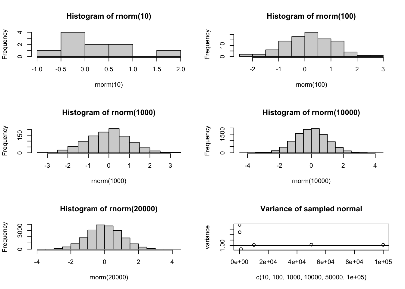
# We're going to first sample directly from a full distribution uniform # distribution from 0 to 1. How many samples will we need to take? # Let's try a few options and see how well they dopar(mfrow=c(3,2))hist(rnorm(10))hist(rnorm(100))hist(rnorm(1000))hist(rnorm(10000))hist(rnorm(20000))# Now let's plot the sample sizes against the variance of the sample distributionplot(c(10,100,1000,10000,50000,100000),c(var(rnorm(10)), var(rnorm(100)), var(rnorm(1000)), var(rnorm(10000)), var(rnorm(50000)), var(rnorm(100000))),ylab ="variance", main ="Variance of sampled normal" )abline(h =1)
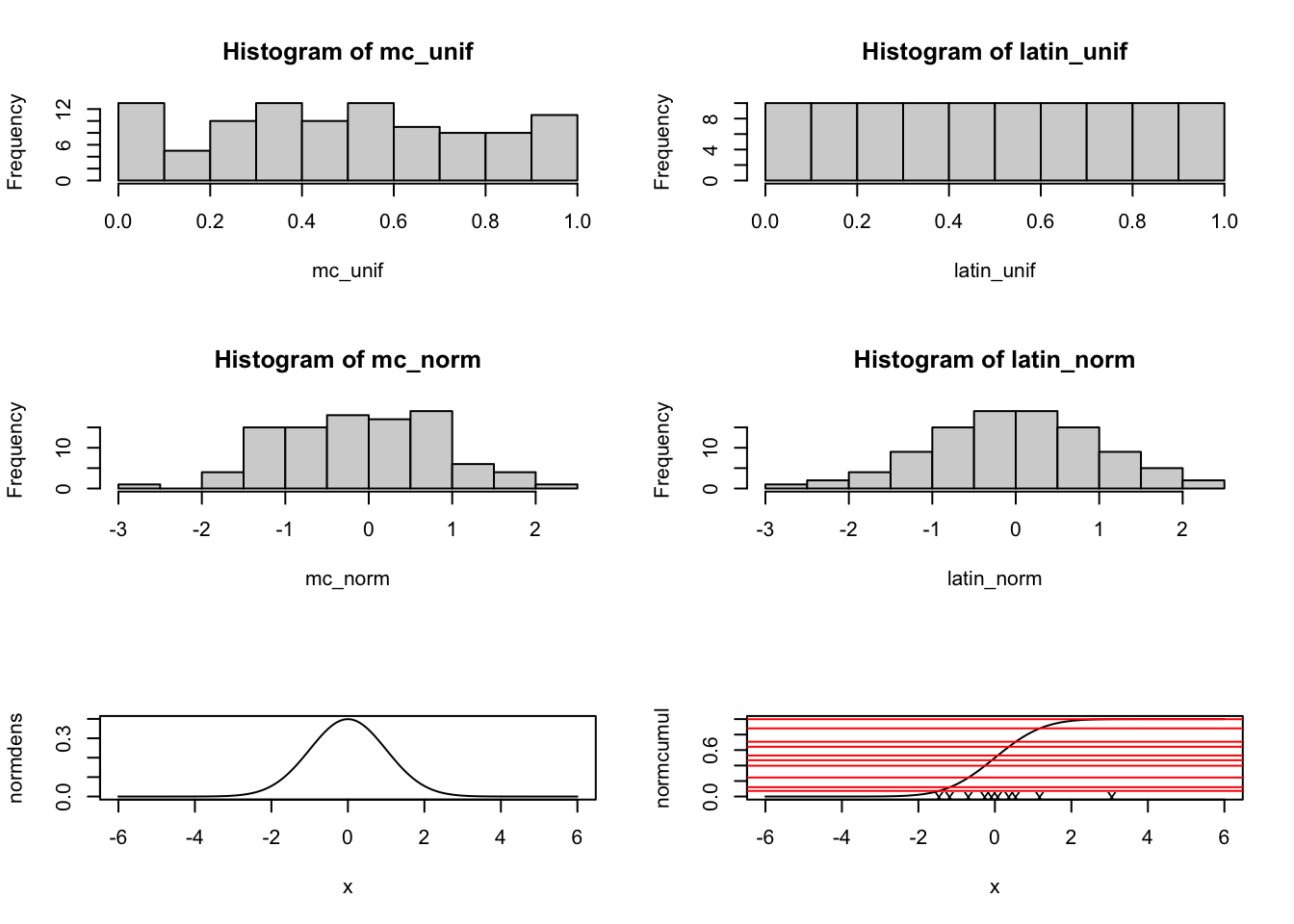
# Let's now use 100 samples to see the difference between a Monte Carlo # sampling and a LHS sampling approach.# Pick some small number of samplesn <-100# First we're going to sample 100 times from a random samplemc_unif <-runif(n)# 100 lh samples across 1 parameterlatin_unif <-randomLHS(n, 1)# plot these two distribution# dev.off()par(mfrow=c(3,2))hist(mc_unif)hist(latin_unif)# You can see how the Latin Hypercube does a great job of sampling evenly # across the distribution. Let's now sample from a Normal distribution using # a random monte carlo sample across the whole distribution.mc_norm <-rnorm(n, mean =0, sd =1)# How do we sample using an LHS? We use the previous numbers generated from the # uniform LHS to draw samples from the Normal using the Inverse Cumulative # Sampling.latin_norm <-qnorm(latin_unif, mean =0, sd =1)# plot these two normal distributionshist(mc_norm)hist(latin_norm)# the latin hypercube sample looks much better! Why does this work?# first let's look at the norm probability distibutionx <-seq(-6, 6, by =0.1) # random variable Xnormdens <-dnorm(x, mean =0, sd =1) # prob distribution, f(X)normcumul <-pnorm(x, mean =0, sd =1) # cumulative distribution, F(X)plot(x, normdens, "l")plot(x, normcumul, "l")# Most of the density is in the middle range of values (-1 to 1).# So we want a method to sample from this more often than the other areas in # the distribution. Specifically, we want to sample values from X proportionally # to the probability of those values occuring. Let's generate some samples # between 0-1. These can be values on our Y-axis. Then, if we ask what is the # value of the cumulative distribution that corresponds to these uniform # values we are taking the inverse for illustration let's just choose 10 points.ex_latin <-randomLHS(10, 1)# which X values are given by using these as the Y value (denoted by "X"s)?abline(h = ex_latin, col ="red")points(qnorm(ex_latin, mean =0, sd =1), y=rep(0,10), pc ="x")
You can see that the samples are clustered around the middle: in areas of X with higher density, the gradient of the cumluative distribution (F(X)) will be very steep, causing more values between 0 and 1 to map to this range of X with high density That is, \(F^{-1}(R) = X\) where R is a uniform random number between 0 and 1.
So, you can sample from any distribution whose cumluative function is ‘invertable’ by plugging in uniform random numbers to the inverse cumulative function of your new distribution. For more information check out: https://en.wikipedia.org/wiki/Inverse_transform_sampling
Likewise, to perform LHS on a uni- or mulitvariate non-uniform distribution, we can transform our LHS samples from a uniform distribution as above.