09. Networks (solutions)

Practical 1. Introduction to the igraph package

library(igraph) # For network functionality
library(data.table)
library(ggplot2)

1. Building and plotting graphs

# Complete graph with 4 nodes
gr <- make_full_graph(4)
print(gr)

IGRAPH e377ec4 U--- 4 6 -- Full graph
+ attr: name (g/c), loops (g/l)
+ edges from e377ec4:
[1] 1--2 1--3 1--4 2--3 2--4 3--4

plot(gr)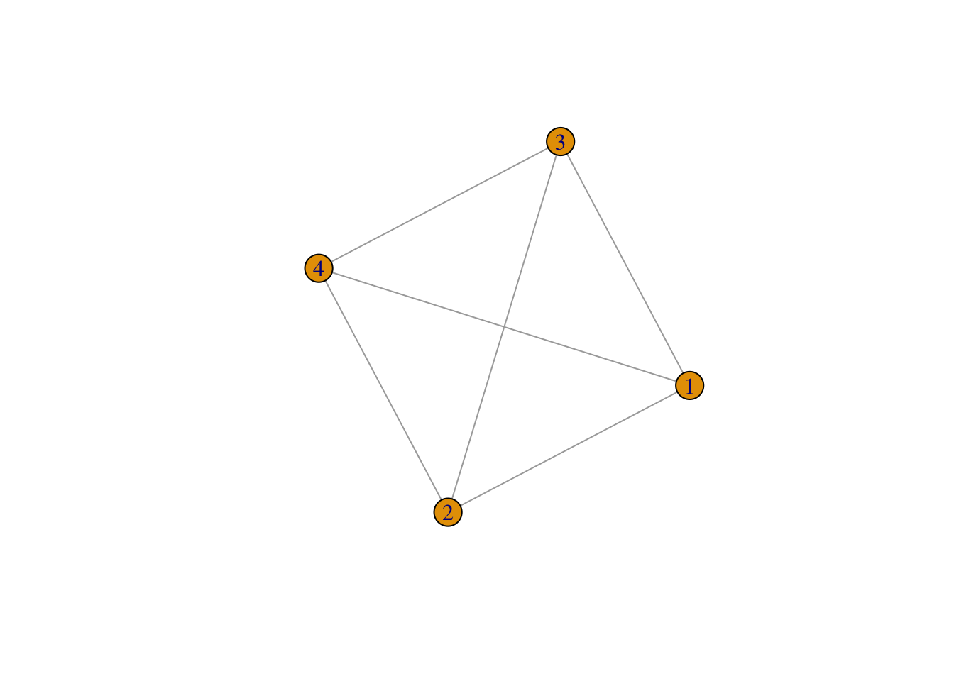

Question (1): Run the plot(gr) line multiple times. The plot changes. Does the graph change?

Answer: The locations of the numbered nodes may change, but the network itself is not changing.

Plot different graphs each with 16 vertices, but different connections between vertices:

gr <- make_full_graph(16)
plot(gr)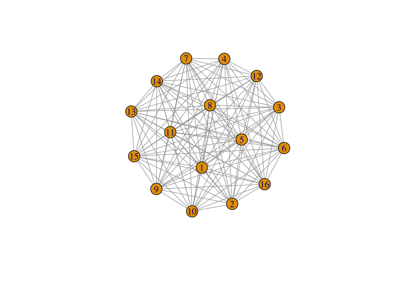

gr <- make_ring(16)
plot(gr)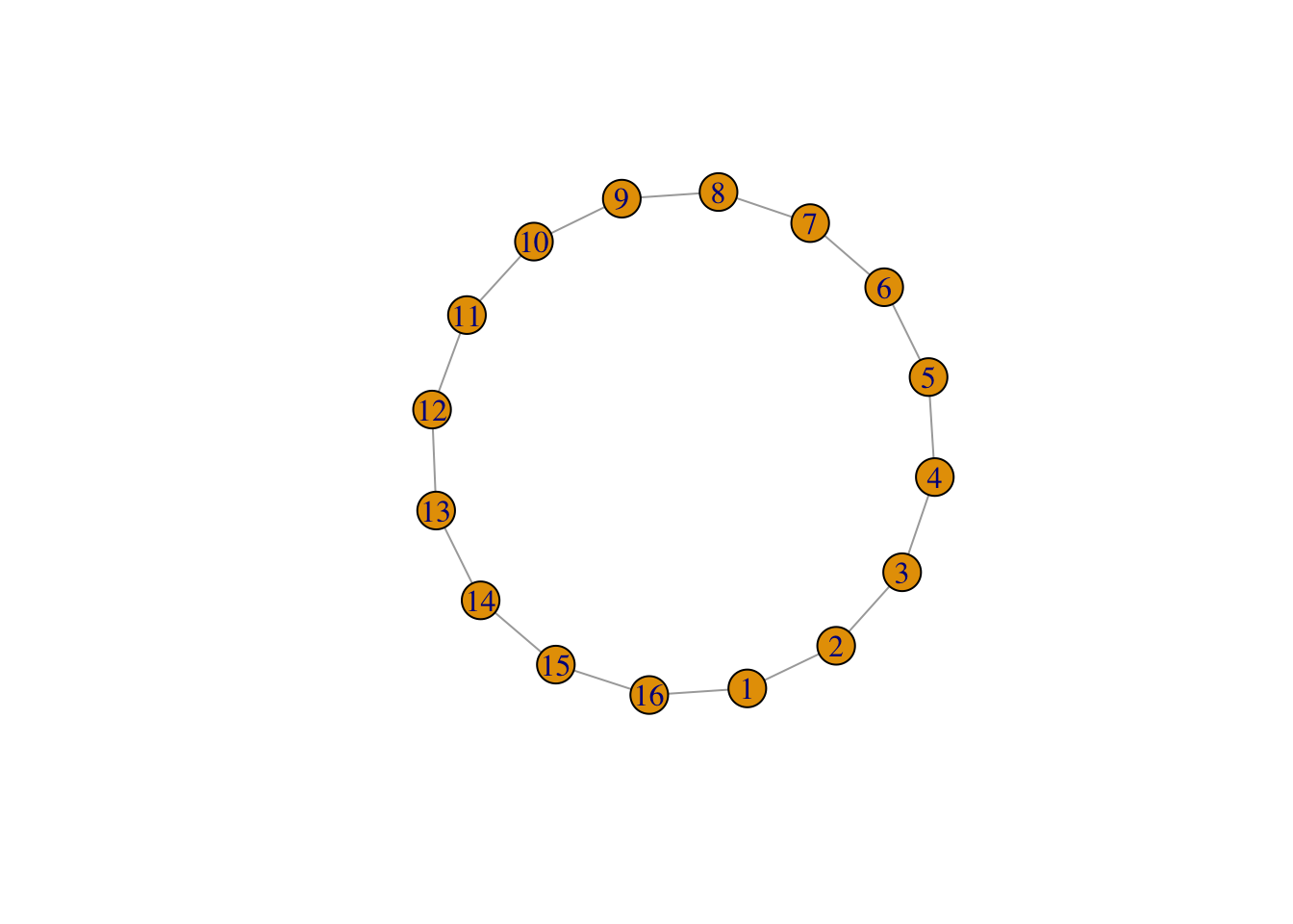

gr <- make_ring(16, circular = FALSE)
plot(gr)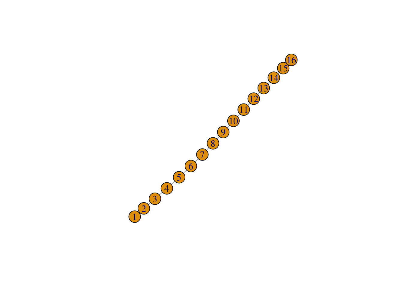

gr <- make_lattice(c(4, 4))
plot(gr)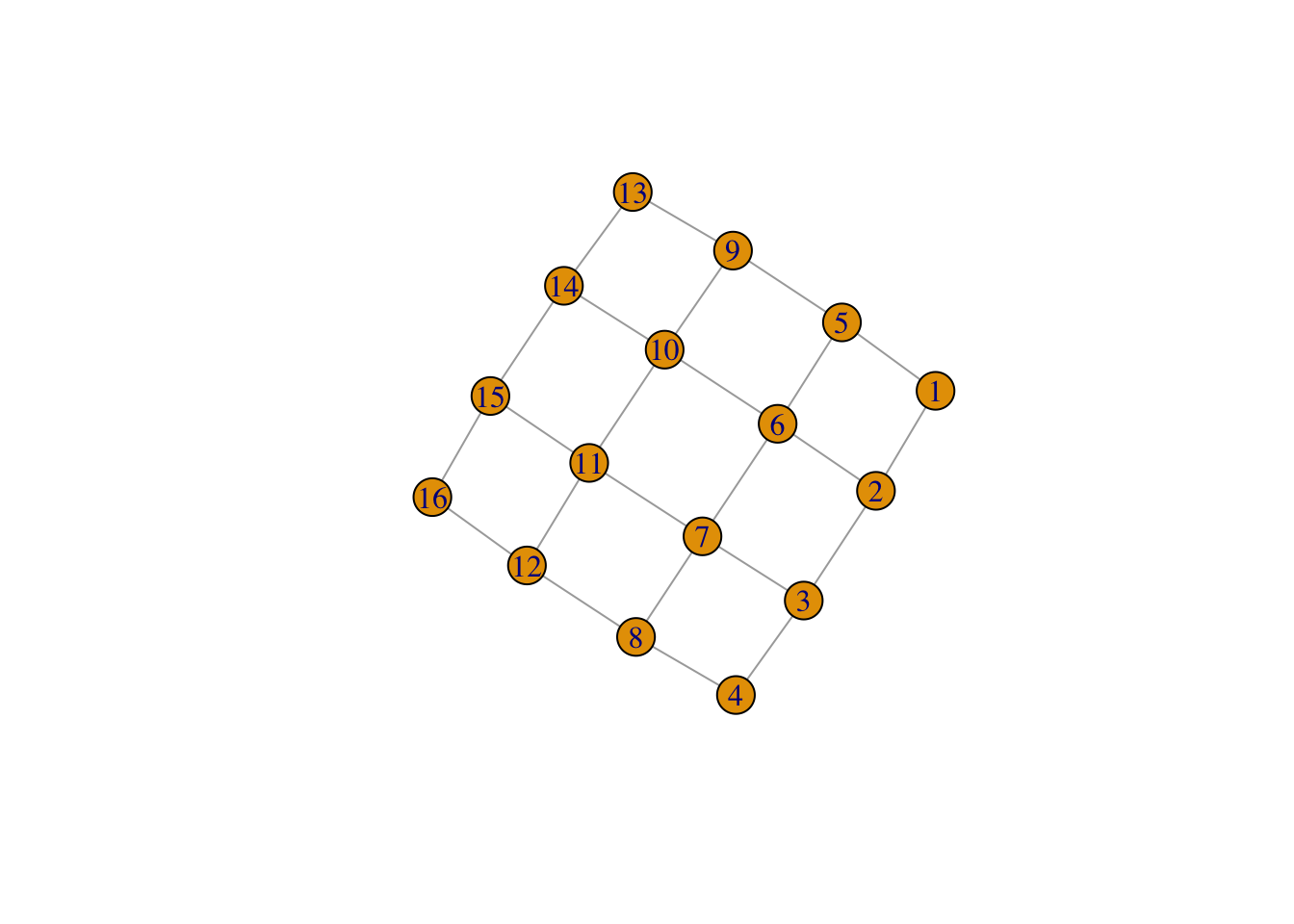

Compare a connected graph with 16 vertices to an Erdős-Rényi G(n, p) graph with 16 vertices:

plot(make_full_graph(16), layout = layout_in_circle)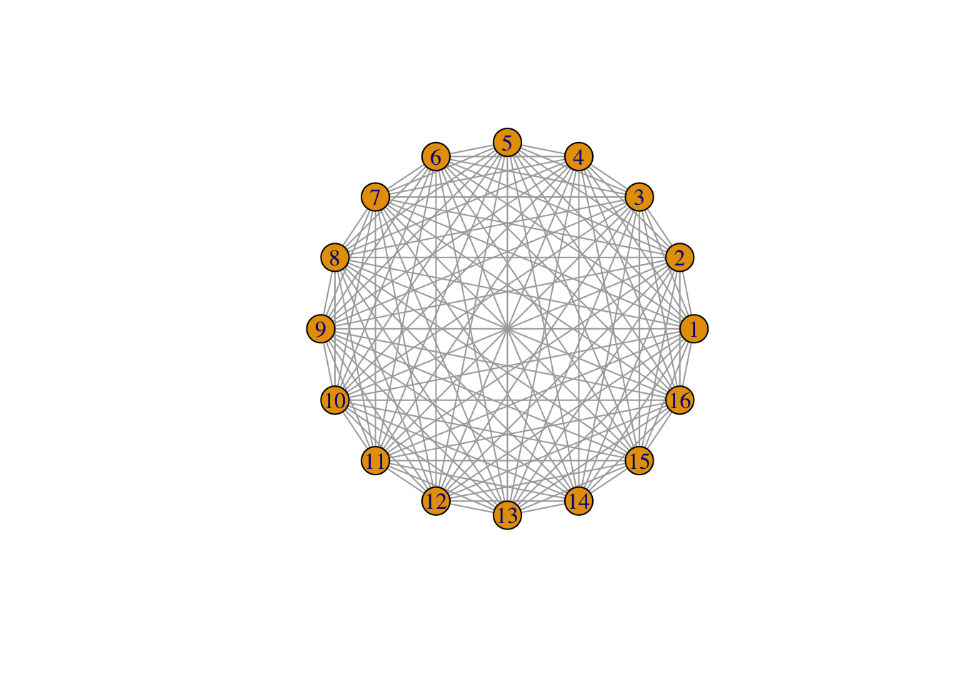

plot(sample_gnp(16, 0.2), layout = layout_in_circle)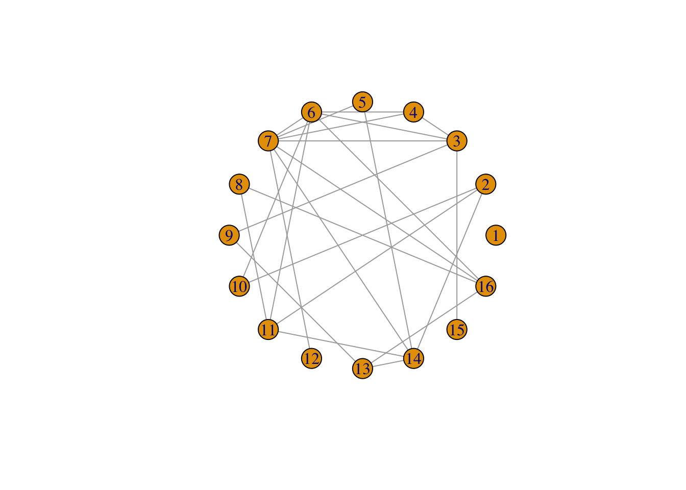

Other random graphs: The “small-world” model by Watts and Strogatz, where there are connections between neighbours, some of which are randomly rewired:

plot(sample_smallworld(1, 16, 2, 0.1), layout = layout_in_circle)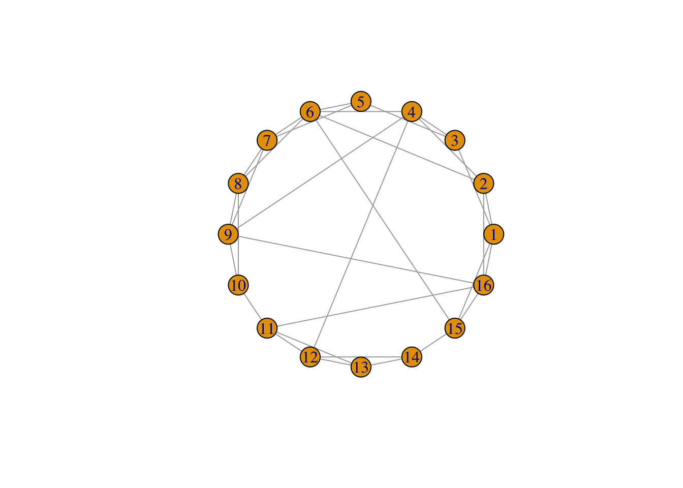

The “preferential attachment” model by Barabási and Albert, which is built by adding nodes one at a time, and each time a node is added, it is connected to other nodes, where the connection is more likely to be made to a node that already has more connections (a “rich get richer” dynamic).

plot(sample_pa(16, directed = FALSE))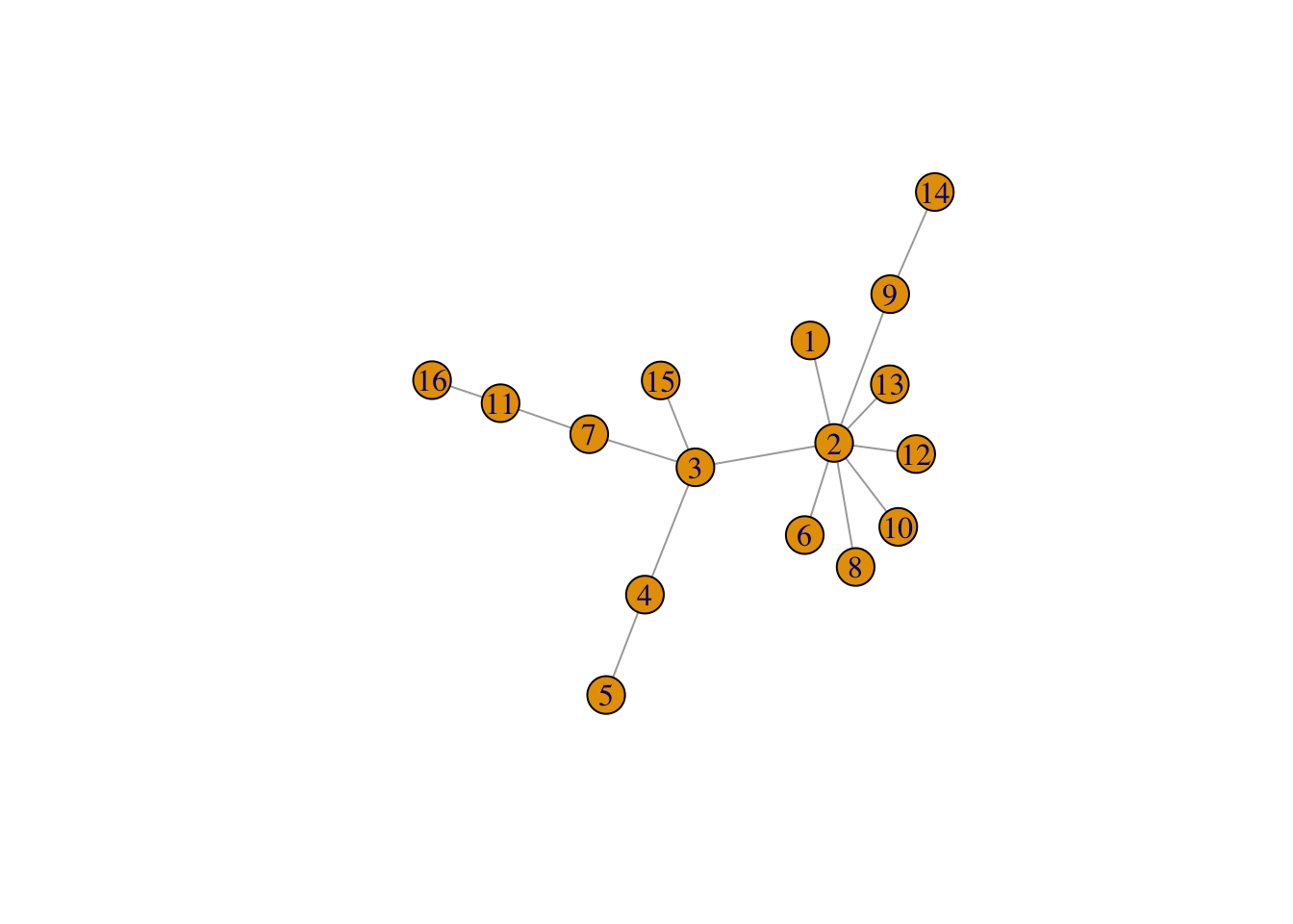

2. Getting and setting properties of the graph

Start by making a new ‘lattice’ graph:

network <- make_lattice(c(5, 5))
print(network)

IGRAPH fa88a6b U--- 25 40 -- Lattice graph
+ attr: name (g/c), dimvector (g/n), nei (g/n), mutual (g/l), circular
| (g/l)
+ edges from fa88a6b:
 [1]  1-- 2  1-- 6  2-- 3  2-- 7  3-- 4  3-- 8  4-- 5  4-- 9  5--10  6-- 7
[11]  6--11  7-- 8  7--12  8-- 9  8--13  9--10  9--14 10--15 11--12 11--16
[21] 12--13 12--17 13--14 13--18 14--15 14--19 15--20 16--17 16--21 17--18
[31] 17--22 18--19 18--23 19--20 19--24 20--25 21--22 22--23 23--24 24--25

plot(network)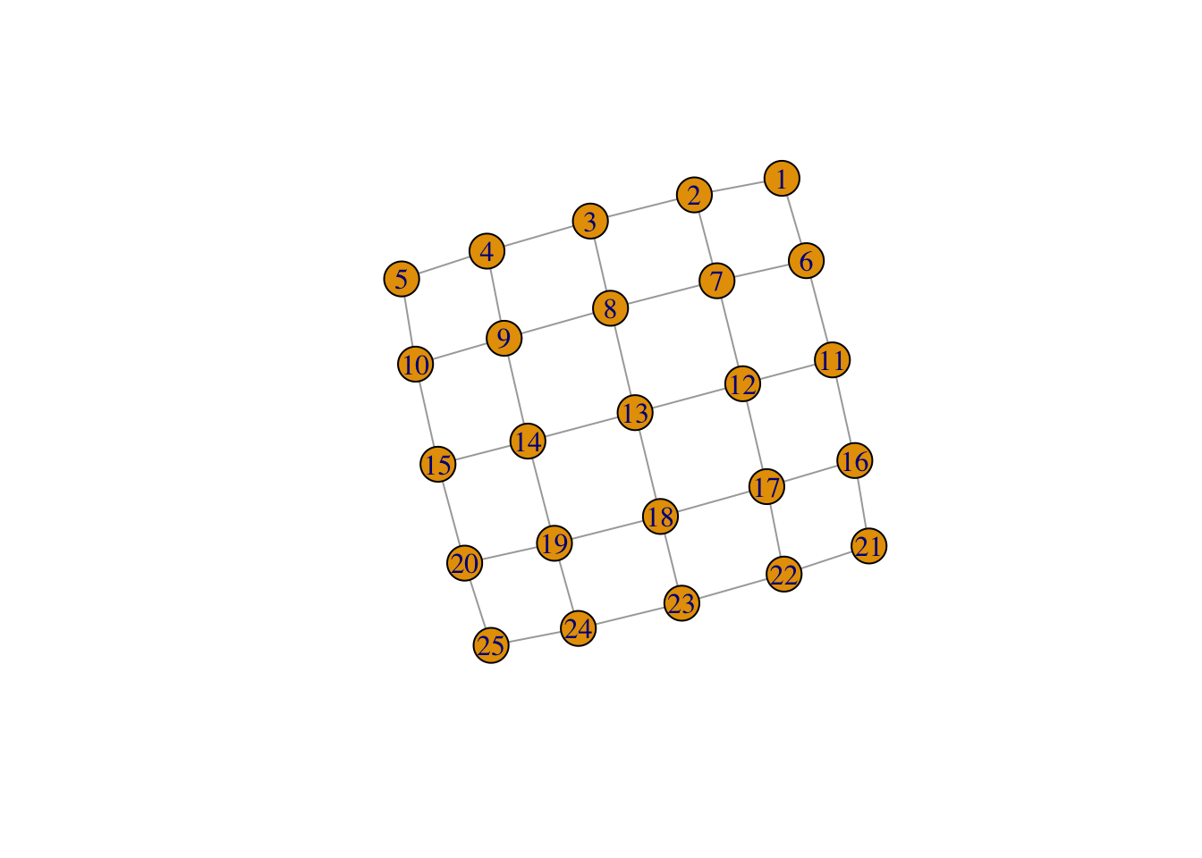

Some simple calculations: vcount() or ecount() give the number of vertices or edges in the graph; degree() gives the number of neighbours of each vertex.

vcount(network)

[1] 25

ecount(network)

[1] 40

degree(network)

 [1] 2 3 3 3 2 3 4 4 4 3 3 4 4 4 3 3 4 4 4 3 2 3 3 3 2

With igraph, you can get and set attributes of the entire graph using the $ operator. For example, let’s set the graph’s layout to a grid:

network$layout <- layout_on_grid(network)
print(network)

IGRAPH fa88a6b U--- 25 40 -- Lattice graph
+ attr: name (g/c), dimvector (g/n), nei (g/n), mutual (g/l), circular
| (g/l), layout (g/n)
+ edges from fa88a6b:
 [1]  1-- 2  1-- 6  2-- 3  2-- 7  3-- 4  3-- 8  4-- 5  4-- 9  5--10  6-- 7
[11]  6--11  7-- 8  7--12  8-- 9  8--13  9--10  9--14 10--15 11--12 11--16
[21] 12--13 12--17 13--14 13--18 14--15 14--19 15--20 16--17 16--21 17--18
[31] 17--22 18--19 18--23 19--20 19--24 20--25 21--22 22--23 23--24 24--25

plot(network)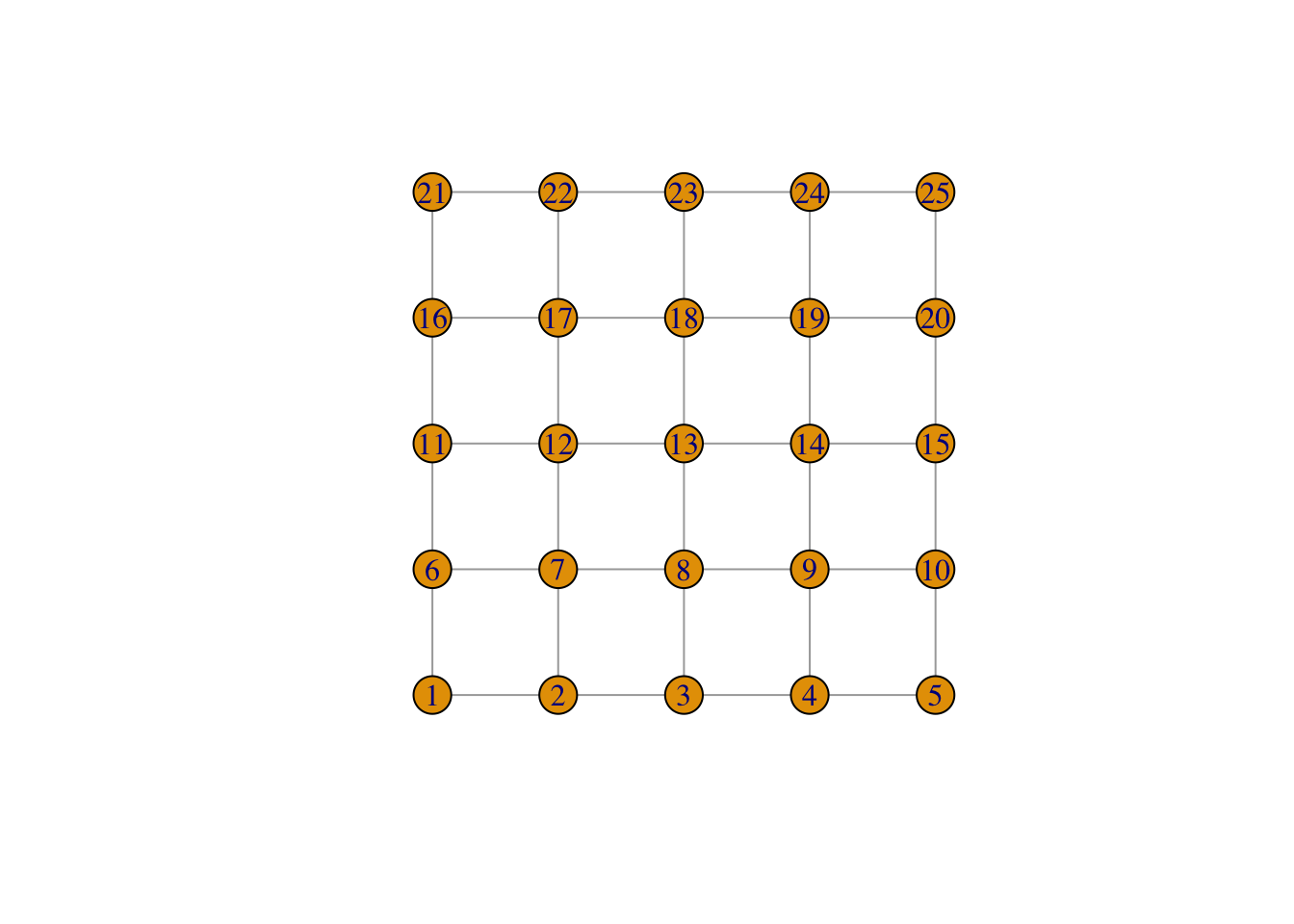

You can also modify properties of the vertices and of the edges, using V() and E() respectively.

V(network)$color <- "azure"
E(network)$color <- "pink"
plot(network) # lovely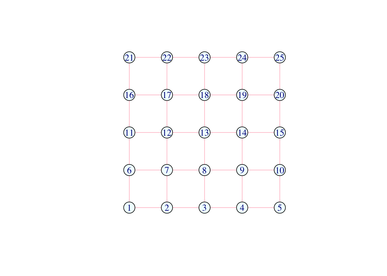

You can use V(network)[[]] or E(network)[[]] to see the properties of the vertices/edges laid out as a data frame:

V(network)[[]]

+ 25/25 vertices, from fa88a6b:
   color
1  azure
2  azure
3  azure
4  azure
5  azure
6  azure
7  azure
8  azure
9  azure
10 azure
11 azure
12 azure
13 azure
14 azure
15 azure
16 azure
17 azure
18 azure
19 azure
20 azure
21 azure
22 azure
23 azure
24 azure
25 azure

E(network)[[]]

+ 40/40 edges from fa88a6b:
   tail head tid hid color
1     1    2   1   2  pink
2     1    6   1   6  pink
3     2    3   2   3  pink
4     2    7   2   7  pink
5     3    4   3   4  pink
6     3    8   3   8  pink
7     4    5   4   5  pink
8     4    9   4   9  pink
9     5   10   5  10  pink
10    6    7   6   7  pink
11    6   11   6  11  pink
12    7    8   7   8  pink
13    7   12   7  12  pink
14    8    9   8   9  pink
15    8   13   8  13  pink
16    9   10   9  10  pink
17    9   14   9  14  pink
18   10   15  10  15  pink
19   11   12  11  12  pink
20   11   16  11  16  pink
21   12   13  12  13  pink
22   12   17  12  17  pink
23   13   14  13  14  pink
24   13   18  13  18  pink
25   14   15  14  15  pink
26   14   19  14  19  pink
27   15   20  15  20  pink
28   16   17  16  17  pink
29   16   21  16  21  pink
30   17   18  17  18  pink
31   17   22  17  22  pink
32   18   19  18  19  pink
33   18   23  18  23  pink
34   19   20  19  20  pink
35   19   24  19  24  pink
36   20   25  20  25  pink
37   21   22  21  22  pink
38   22   23  22  23  pink
39   23   24  23  24  pink
40   24   25  24  25  pink

The “color” attribute is now also listed when we print the network:

network

IGRAPH fa88a6b U--- 25 40 -- Lattice graph
+ attr: name (g/c), dimvector (g/n), nei (g/n), mutual (g/l), circular
| (g/l), layout (g/n), color (v/c), color (e/c)
+ edges from fa88a6b:
 [1]  1-- 2  1-- 6  2-- 3  2-- 7  3-- 4  3-- 8  4-- 5  4-- 9  5--10  6-- 7
[11]  6--11  7-- 8  7--12  8-- 9  8--13  9--10  9--14 10--15 11--12 11--16
[21] 12--13 12--17 13--14 13--18 14--15 14--19 15--20 16--17 16--21 17--18
[31] 17--22 18--19 18--23 19--20 19--24 20--25 21--22 22--23 23--24 24--25

Finally, we can also use brackets [] to change properties of only certain vertices/edges.

V(network)[12]$color <- "orange"
plot(network)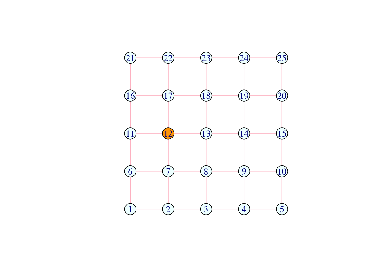

V(network)[color == "orange"]$color <- "pink"
plot(network)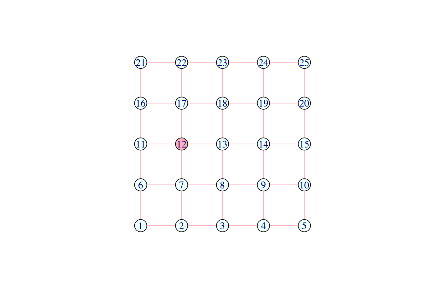

Question (2): What do the above lines do?

Answer: Change the vertex with index 12 into orange. Then change all orange vertices from orange to pink.

Pink is contagious:

V(network)[.nei(color == "pink")]$color <- "pink"
plot(network)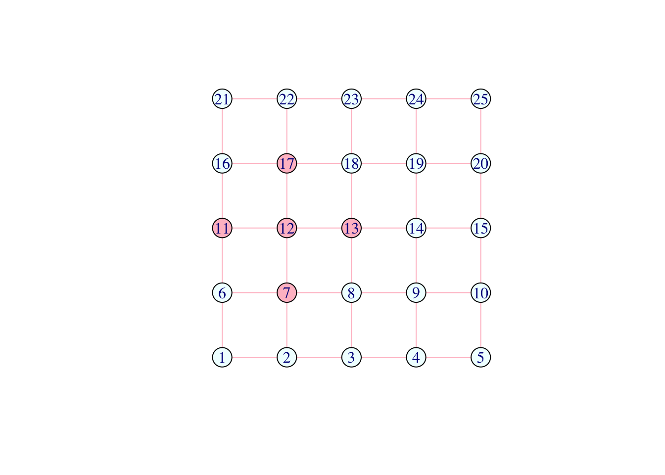

Question (3): What is the code above? What happens if you re-run the last two lines above several times?
Answer: Change the colors of vertices neighboring a pink vertex to pink. The number of pink points in this network gradually increase.

Other interesting attributes for vertices include:

V(network)$label <- NA        # text label for the vertices (set to NA for no labels)
V(network)$size <- 5          # size of vertex markers
V(network)$shape <- "square"  # shape of markers
plot(network)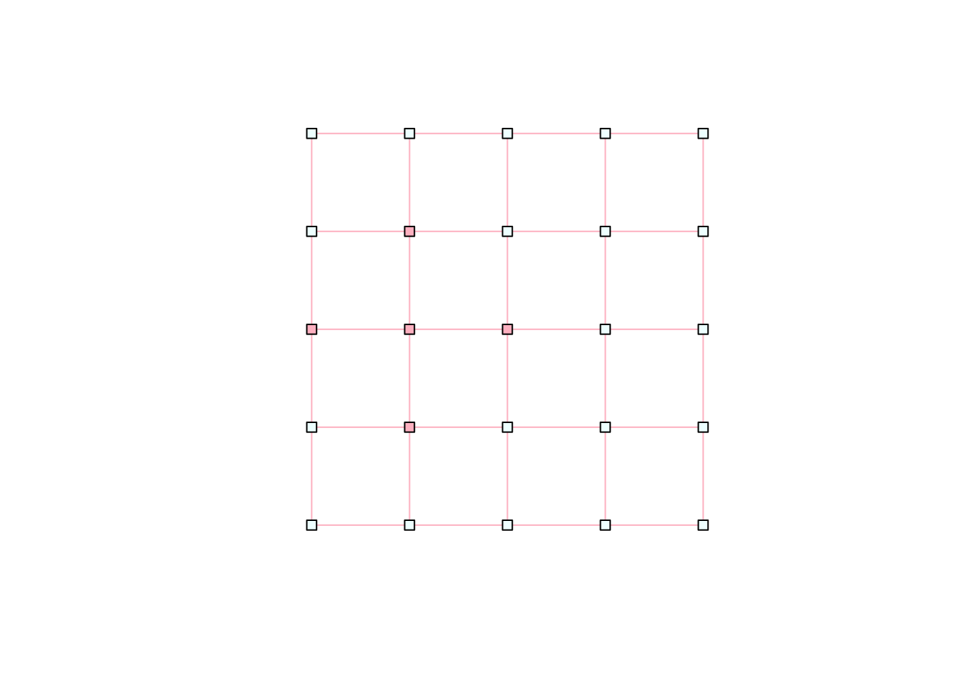

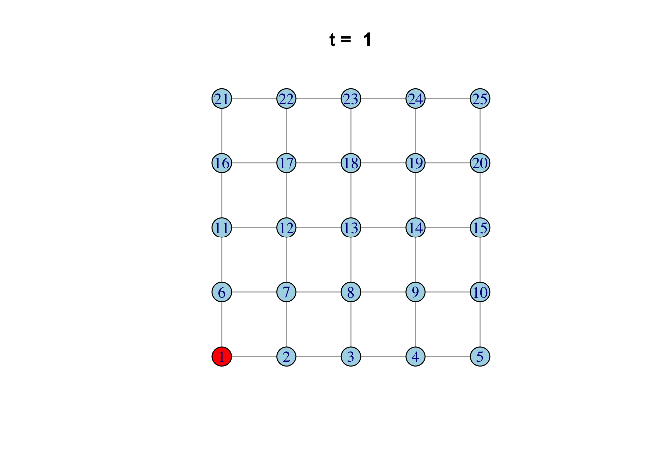
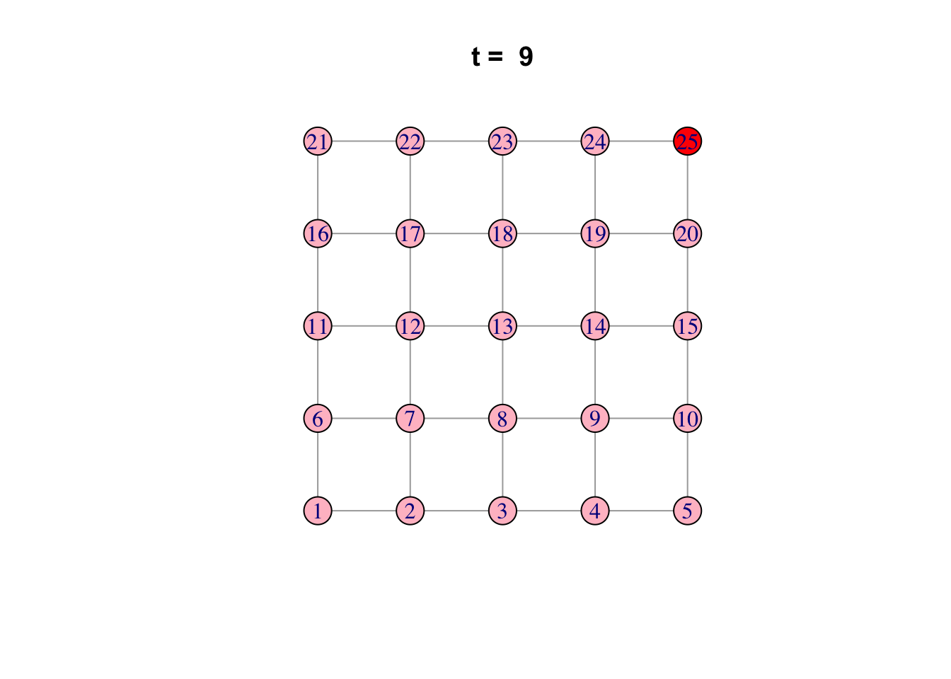
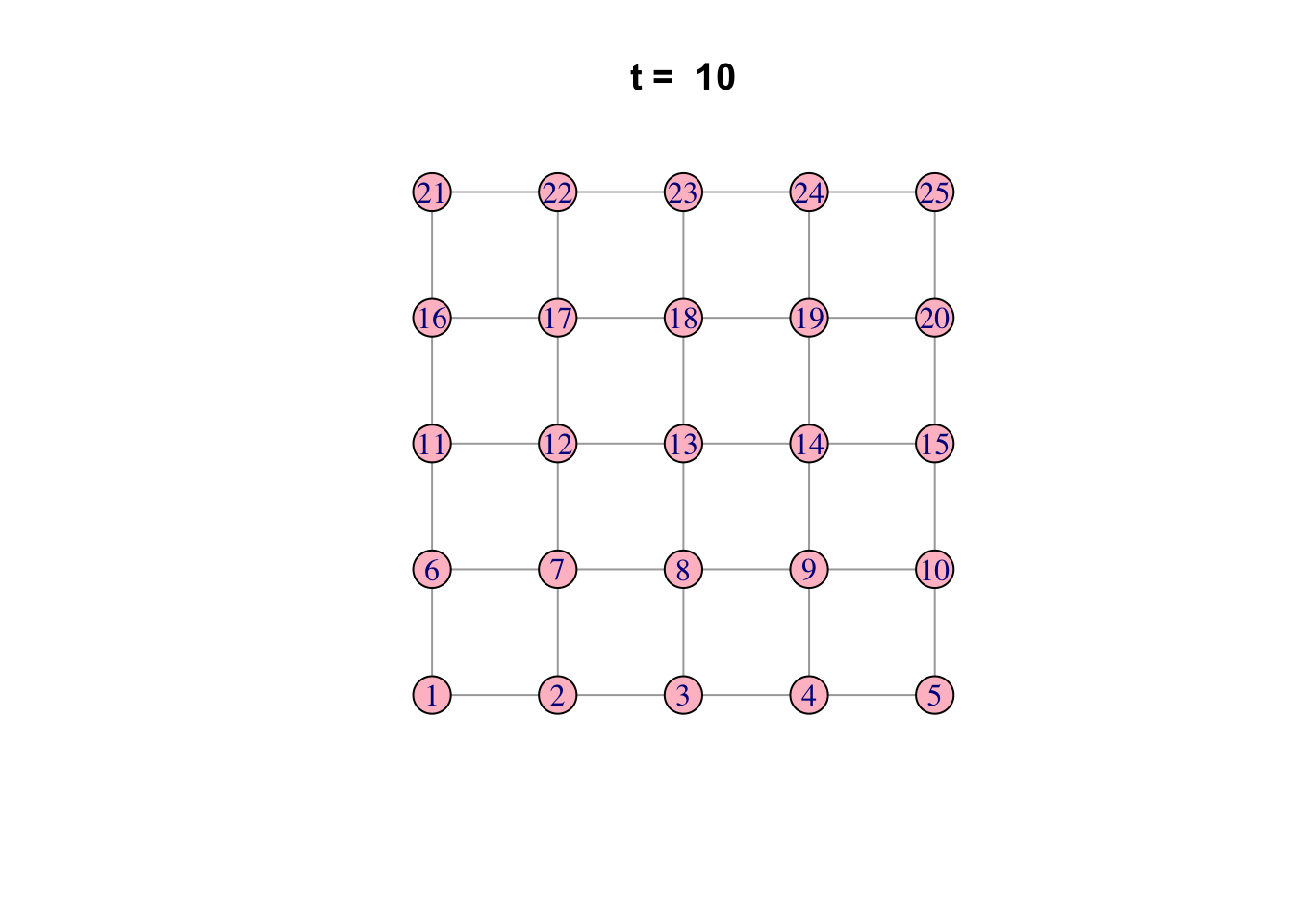
# See ?igraph.plotting for more.

Bonus: Code a network model

Here is one possible way of doing it…

network <- make_lattice(c(5, 5))

Set all vertices to “susceptible” except for one “infected”

V(network)$state <- "S"
V(network)[1]$state <- "I"

# Pick plotting colours
colours <- c(S = "lightblue", I = "red", R = "pink")

# Print and loop through time steps
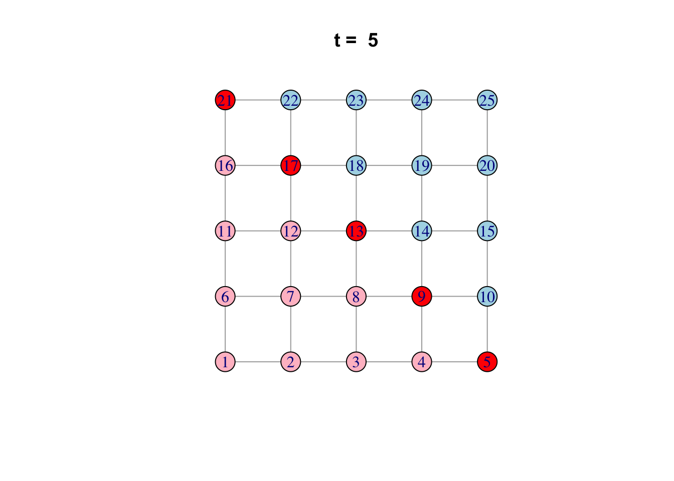
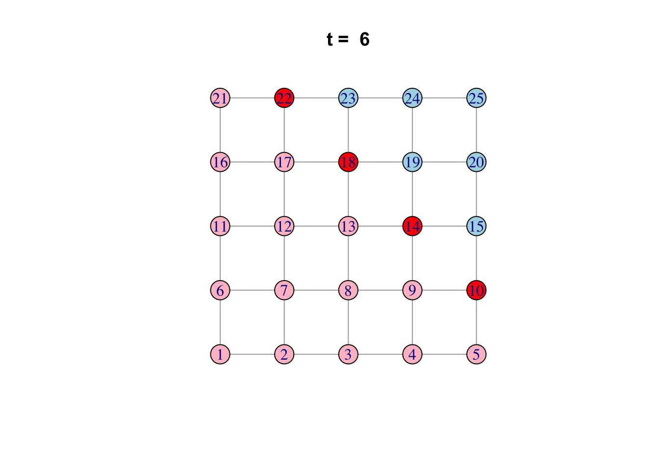
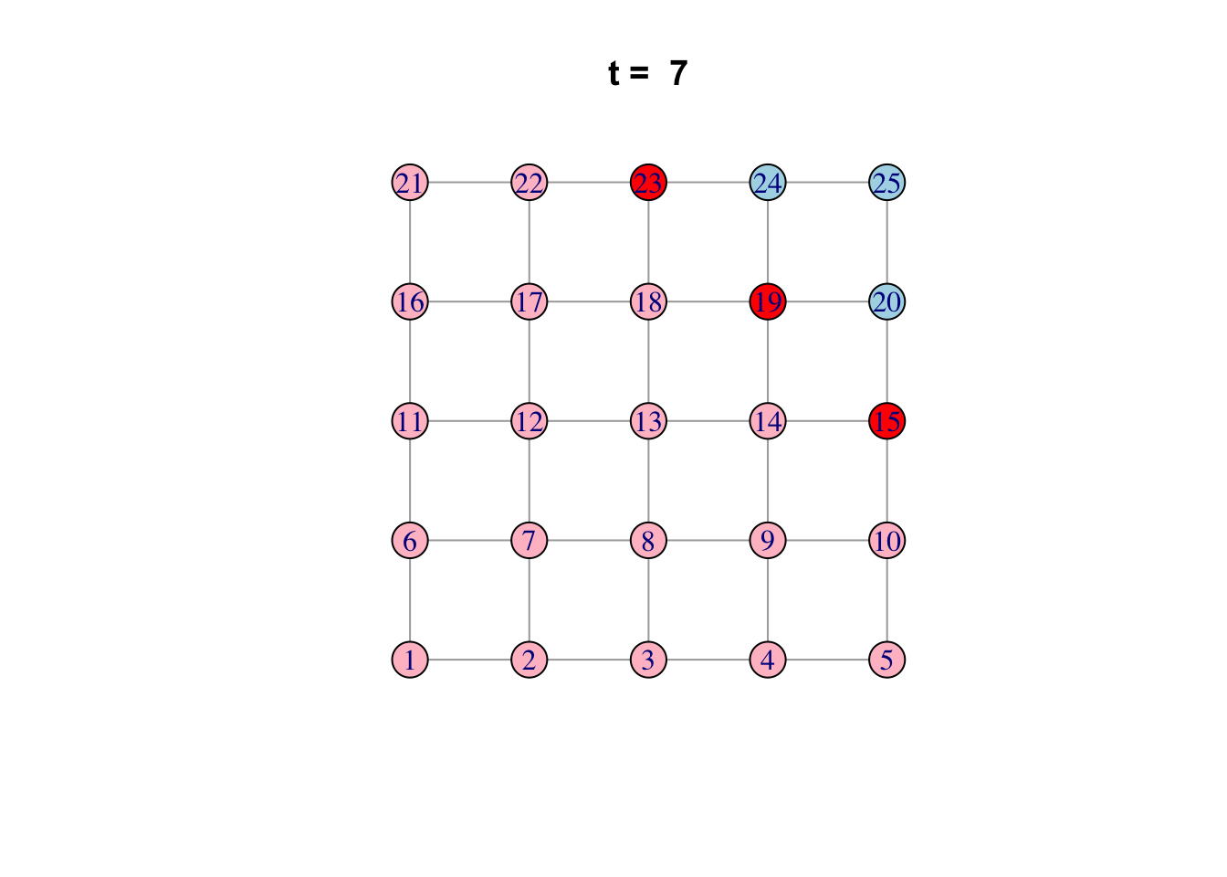
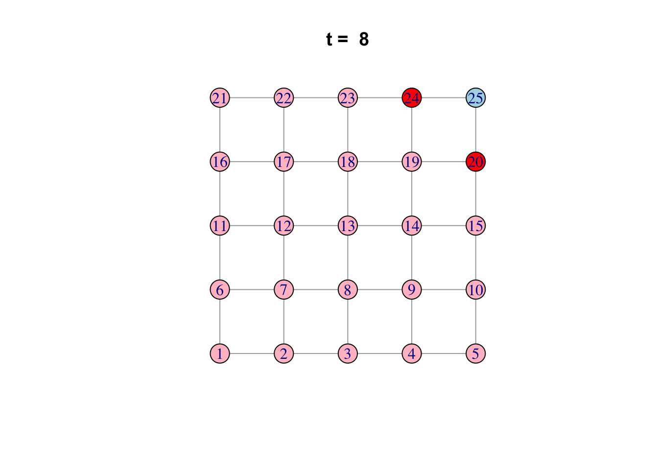
t_max <- 10
for (t in 1:t_max)
{
    # Plot network
    plot(network, 
        vertex.color = colours[V(network)$state], 
        layout = layout_on_grid,
        main = paste("t = ", t))
    
    # Pause so we can see animation
    Sys.sleep(1.0)
    
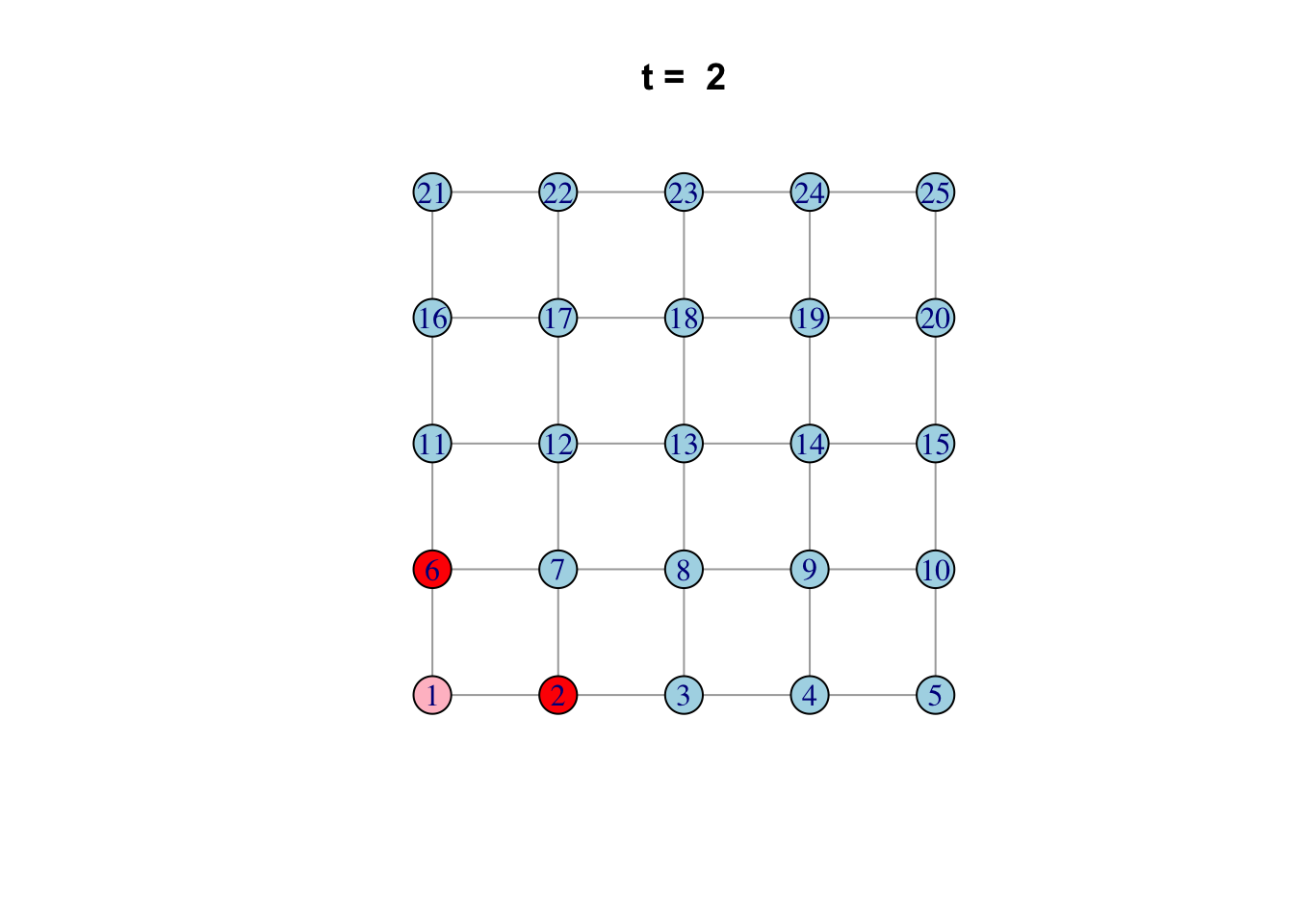
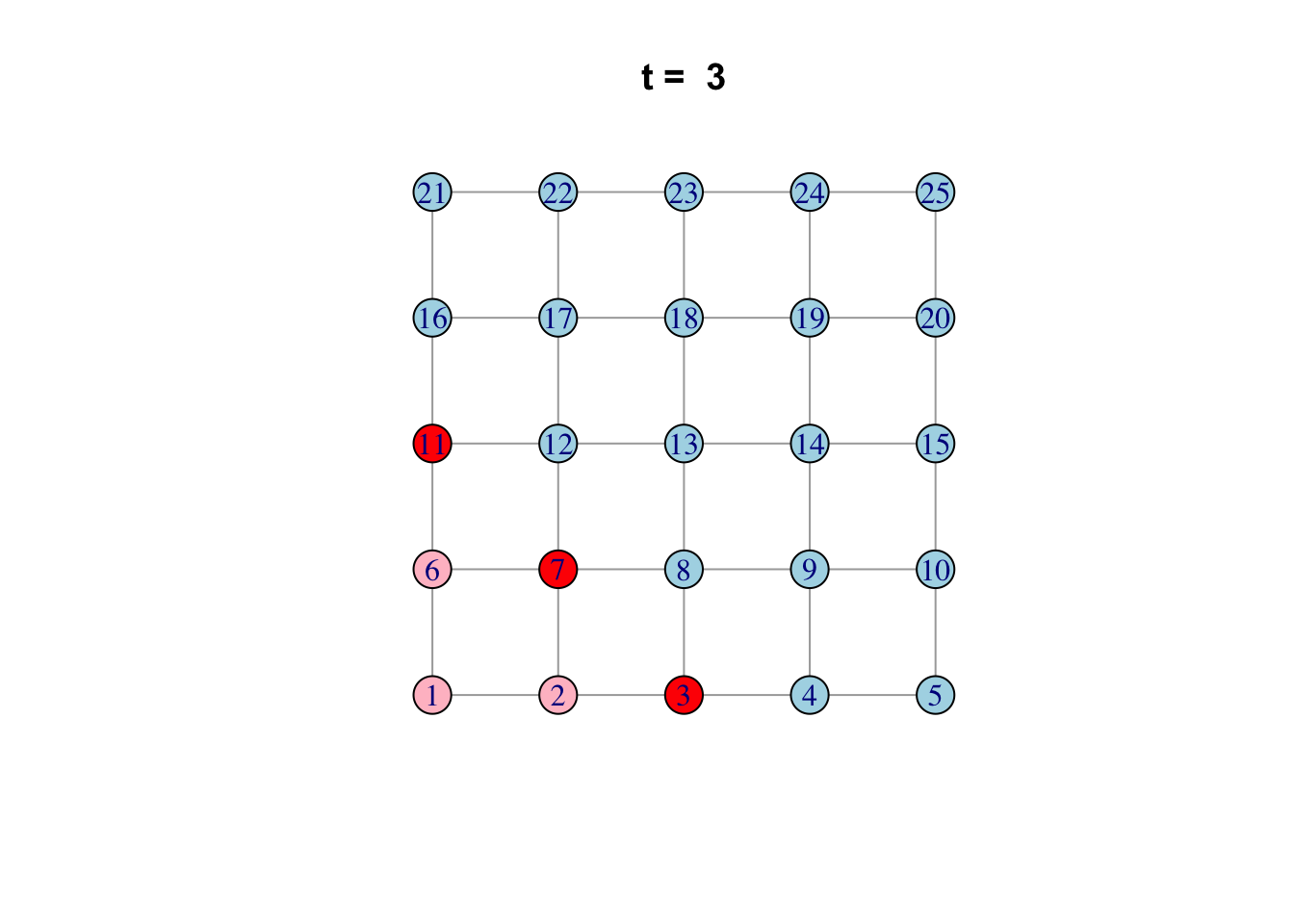
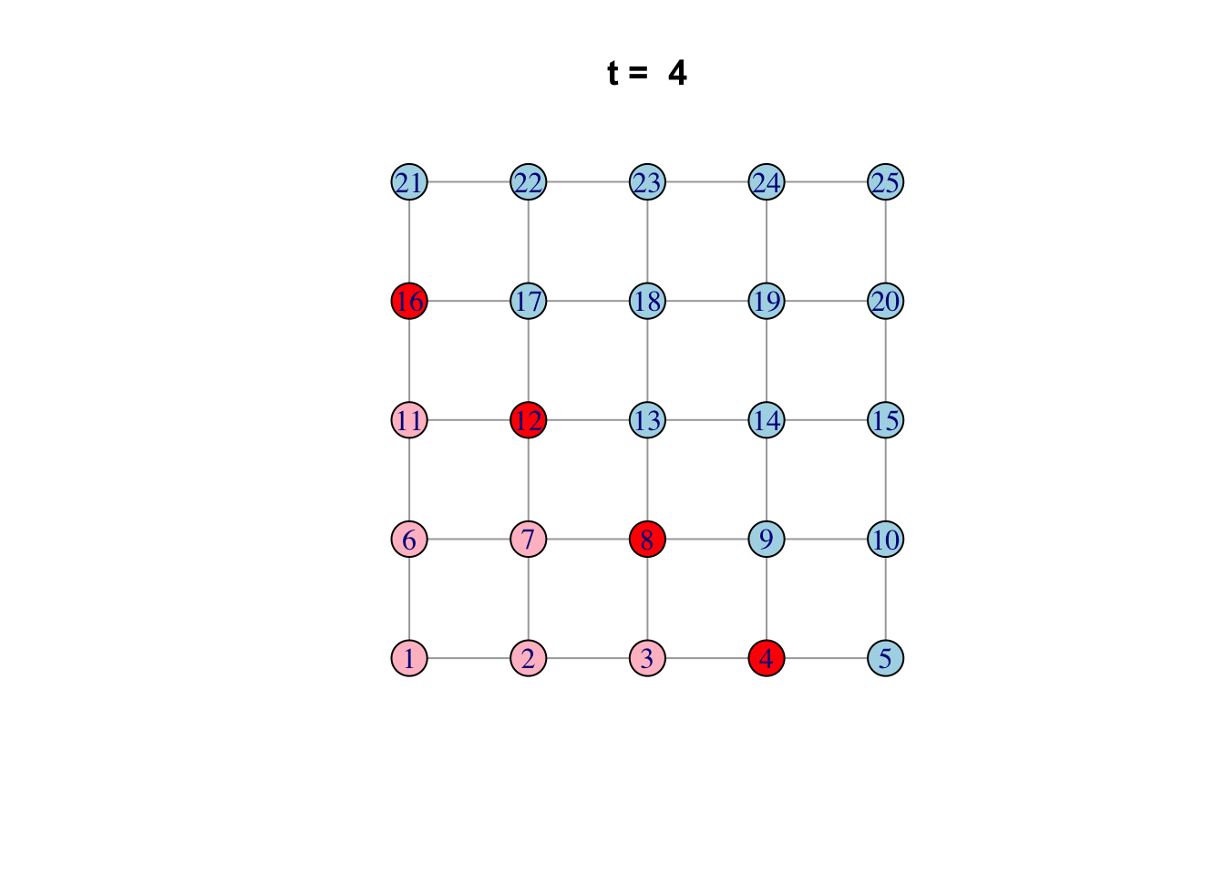
    # Find "infector" vertices
    infectors <- V(network)[state == "I"]
    
    # Infect susceptible neighbours of infectors
    V(network)[.nei(infectors) & state == "S"]$state <- "I"
    
    # Recover infectors
    V(network)[infectors]$state <- "R"
}

Practical 2. A network model of mpox transmission

library(igraph)
library(data.table)
library(ggplot2)

1. Setting up the network

Set up a transmission network of n nodes by preferential attachment with affinity proportional to degree^m.

create_network <- function(n, d, layout = layout_nicely)
{
    # Create the network by preferential attachment, 
    # passing on the parameters n and power
    network <- sample_pa(n, d, directed = FALSE)

    # Add the "state" attribute to the vertices of 
    #the network, which can be "S", "I", "R", or "V". 
    # Start out everyone as susceptible ...
    V(network)$state <- "S"
    
    # ... except make 5 random individuals infectious.
    V(network)$state[sample(vcount(network), 5, prob = degree(network))] <- "I"

    # Reorder vertices so they go in order from least to most connected. This
    # is to help with degree-targeted vaccination, and also to make the 
    # most connected vertices plot on top so they don't get hidden. 
    network <- permute(network, rank(degree(network), ties.method = "first"))
    # Set the network layout so it doesn't change every time it's plotted.
    network$layout <- layout(network)
    
    return (network)
}

## See how the parameter d to create_network changes the network structure
net <- create_network(40, 0)
plot(net)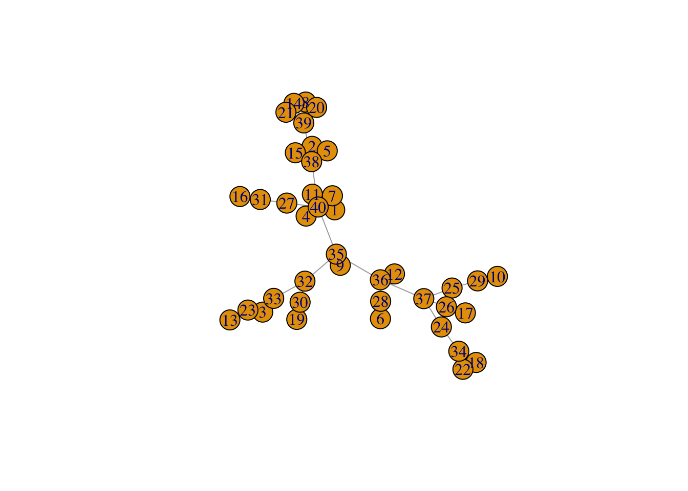

net <- create_network(40, 1)
plot(net)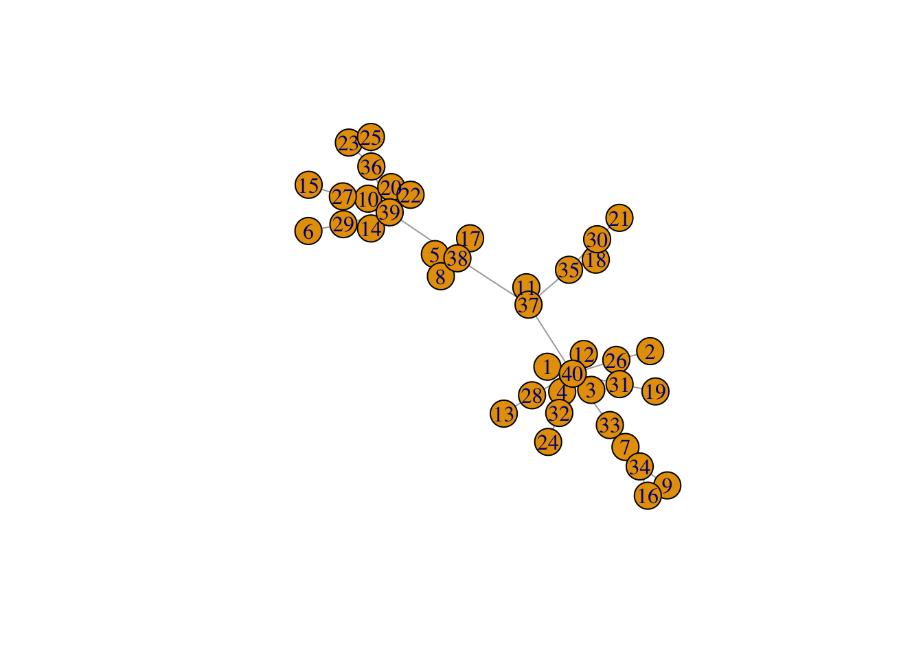

net <- create_network(40, 2)
plot(net)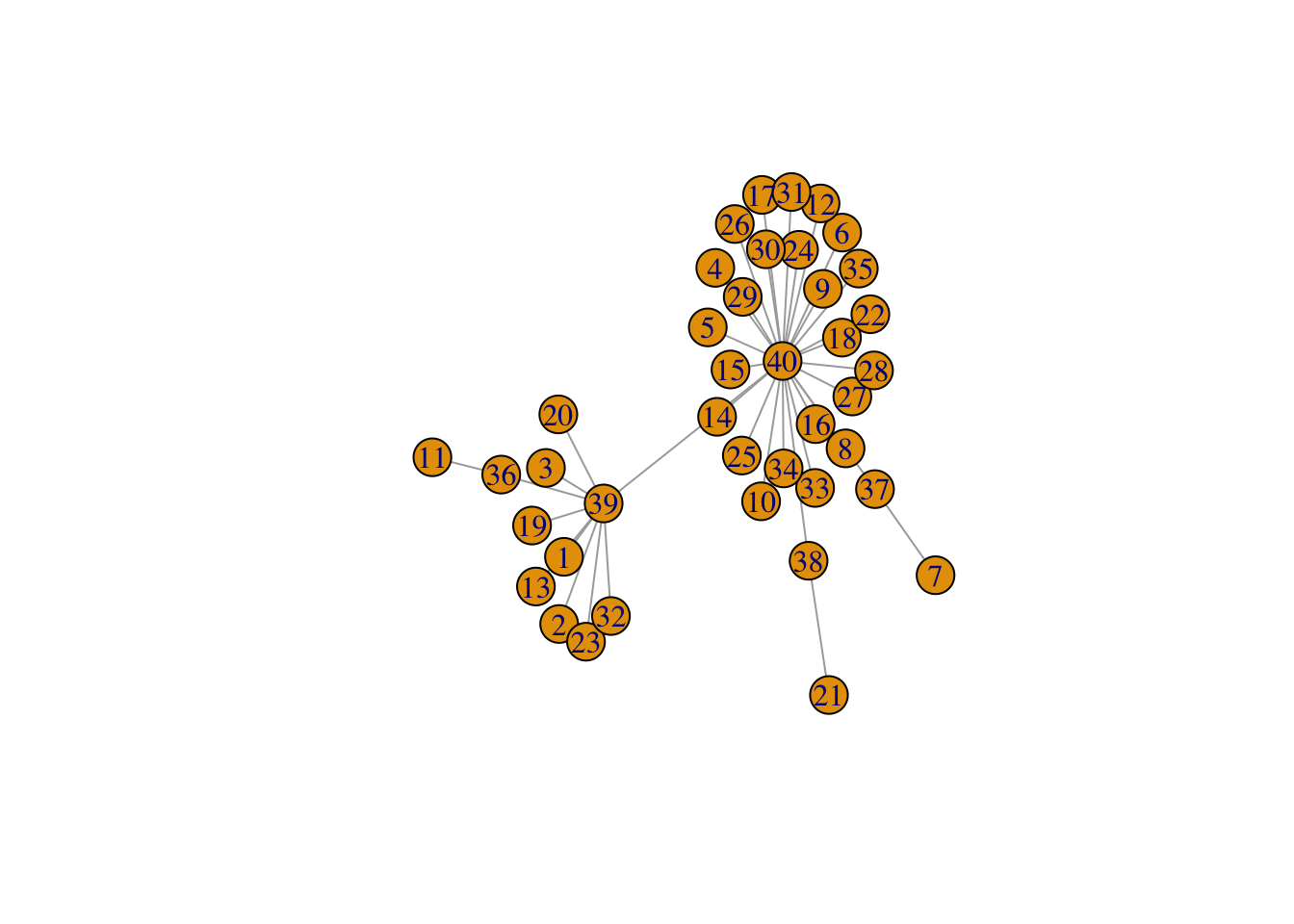

Question (1): Try varying the d parameter for create_network between 0 and 2. What changes about the network?

Answer: All vertices are increasingly connected through the same vertex.

Plot a network, highlighting the degree of each node by different colours.

plot_degree <- function(network)
{
    # Set up palette
    colors <- hcl.colors(5, "Zissou 1")
    
    # Classify nodes by degree
    deg <- cut(degree(network), 
        breaks = c(1, 2, 5, 10, 20, Inf),
        labels = c("1", "2-4", "5-9", "10-19", "20+"),
        include.lowest = TRUE, right = FALSE)

    # Plot network
    plot(network, 
        vertex.color = colors[deg],
        vertex.label = NA,
        vertex.size = 4)
    legend("topright", levels(deg), fill = colors, title = "Degree")
}

## Look at the degree distribution plotted for different values of d
net <- create_network(500, 1)
plot_degree(net)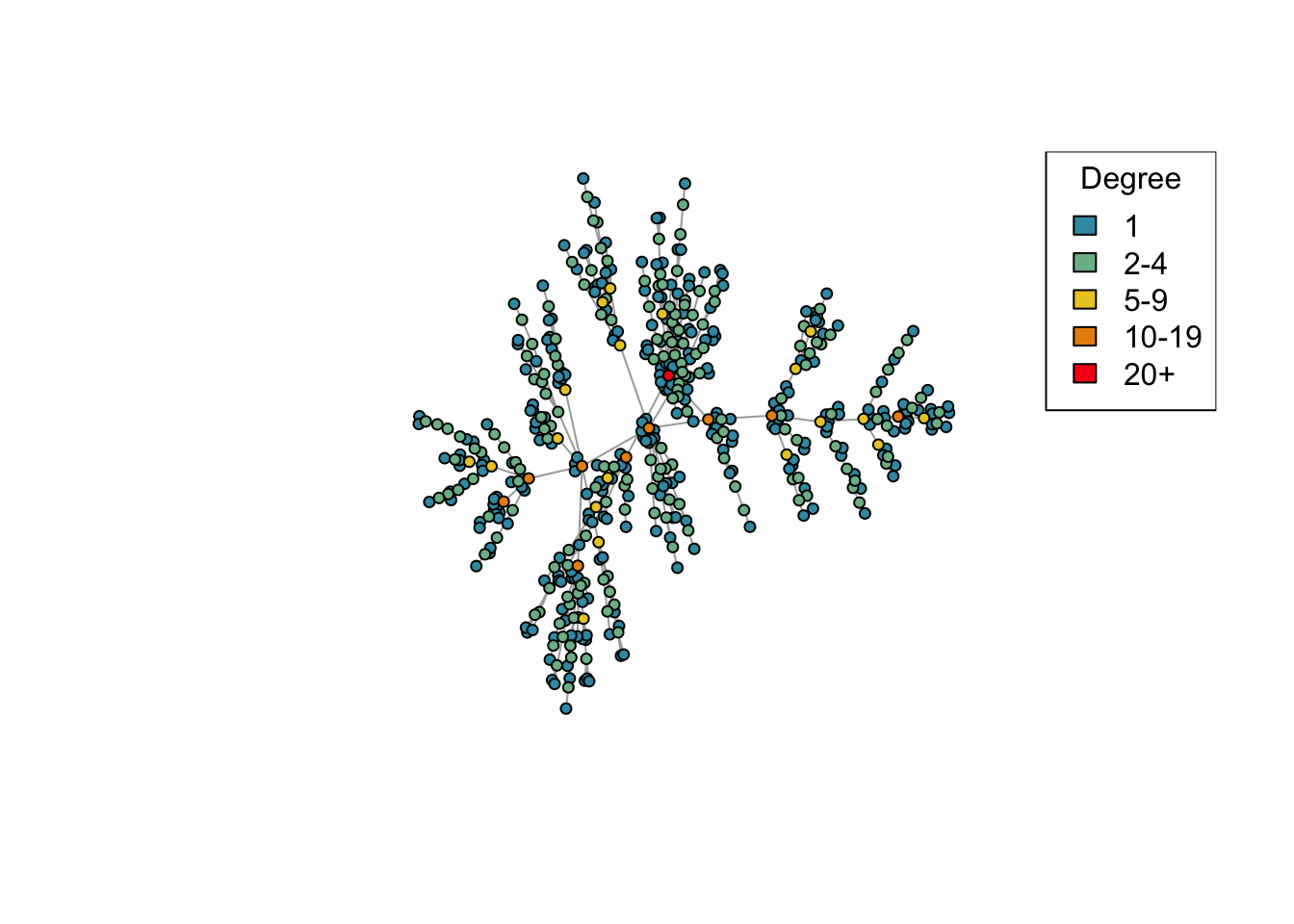

net <- create_network(500, 1.5)
plot_degree(net)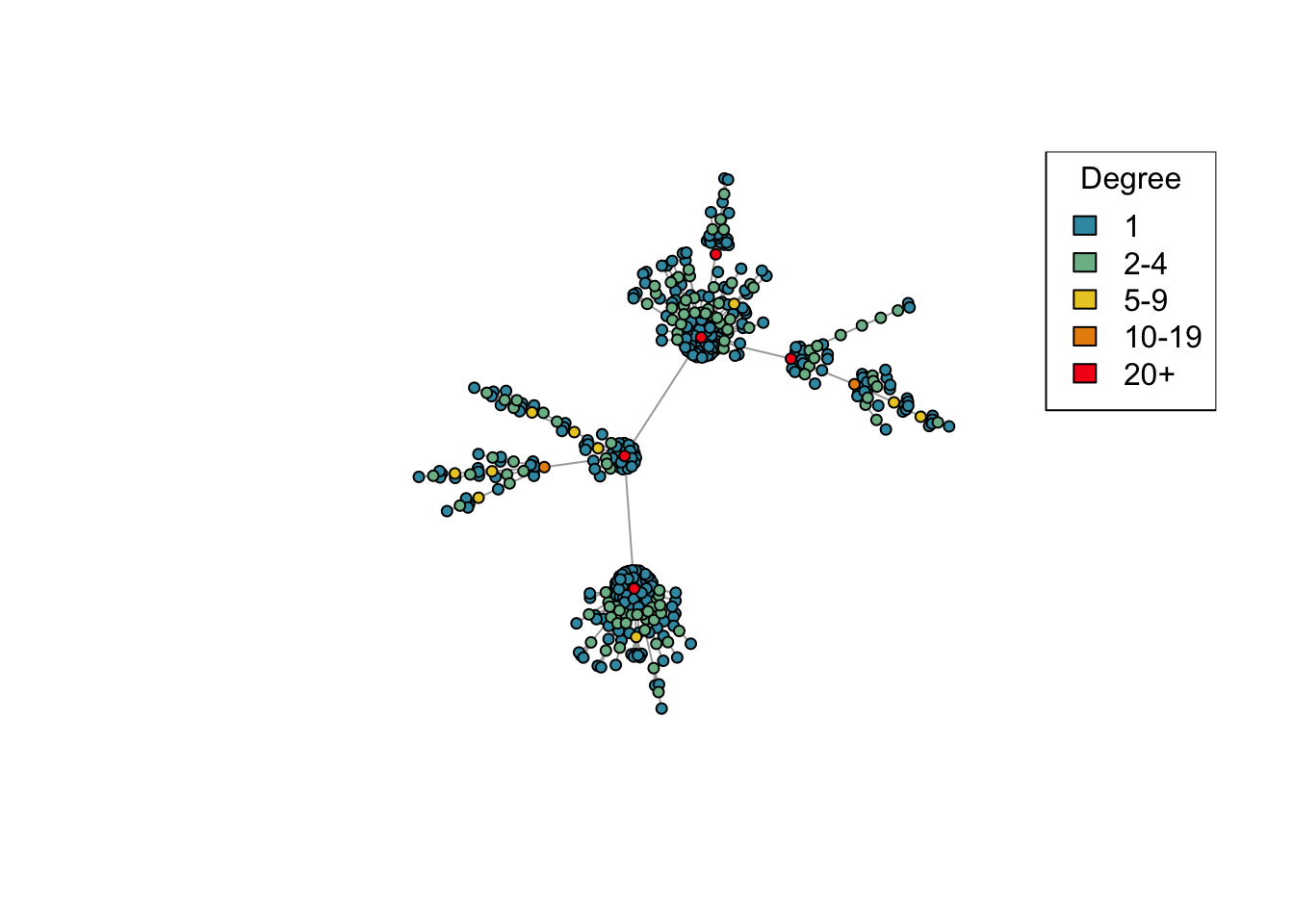

net <- create_network(500, 2)
plot_degree(net)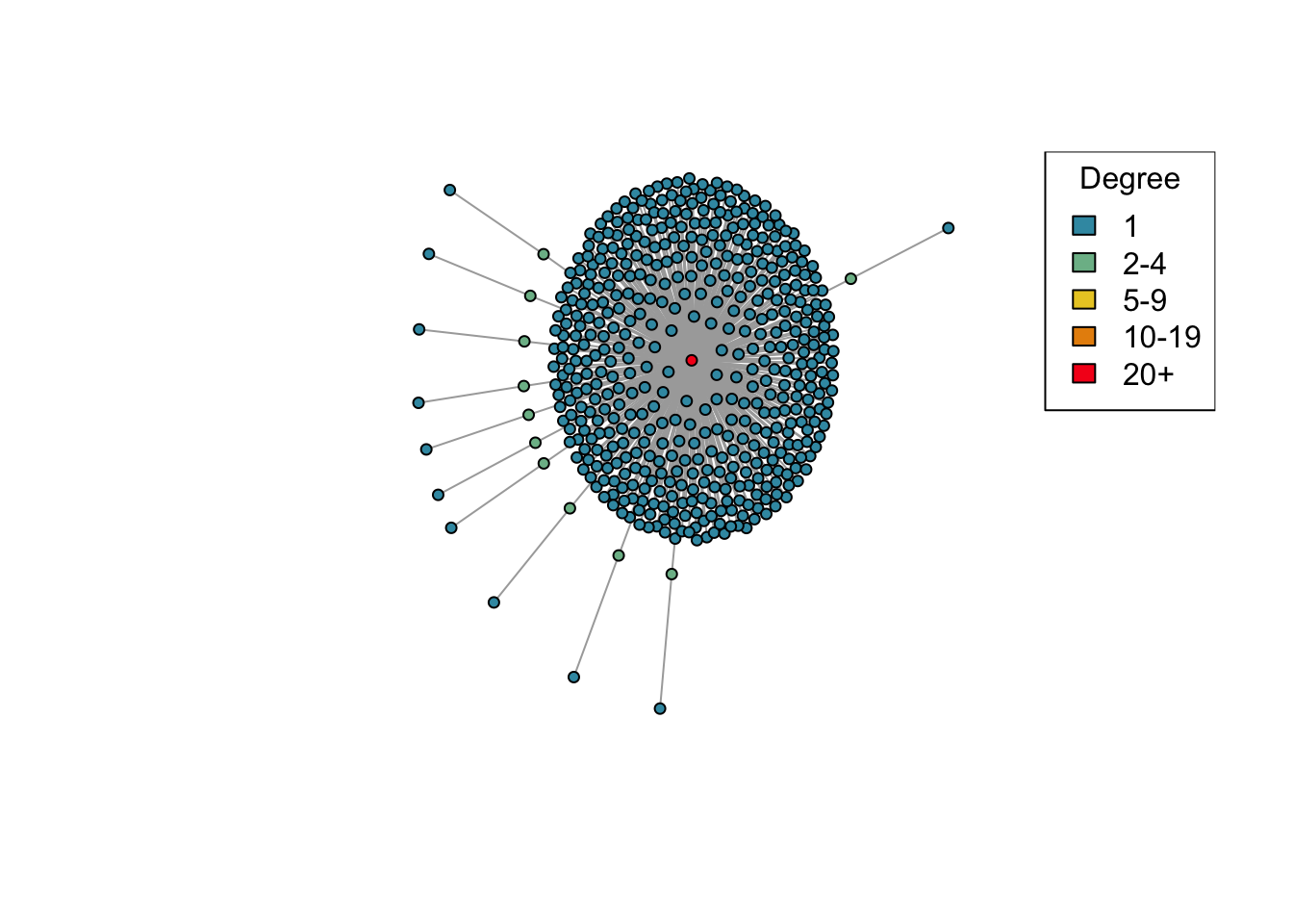

Question (2): This time we’ve created a network with 500 nodes. Try varying the d parameter again and plotting the generated networks. Are the results similar to what you saw before with 40 nodes?

Answer: Yes.

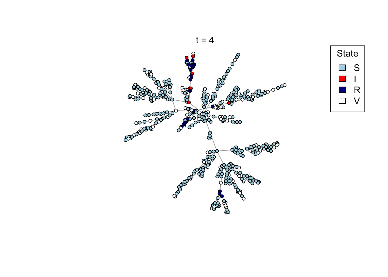
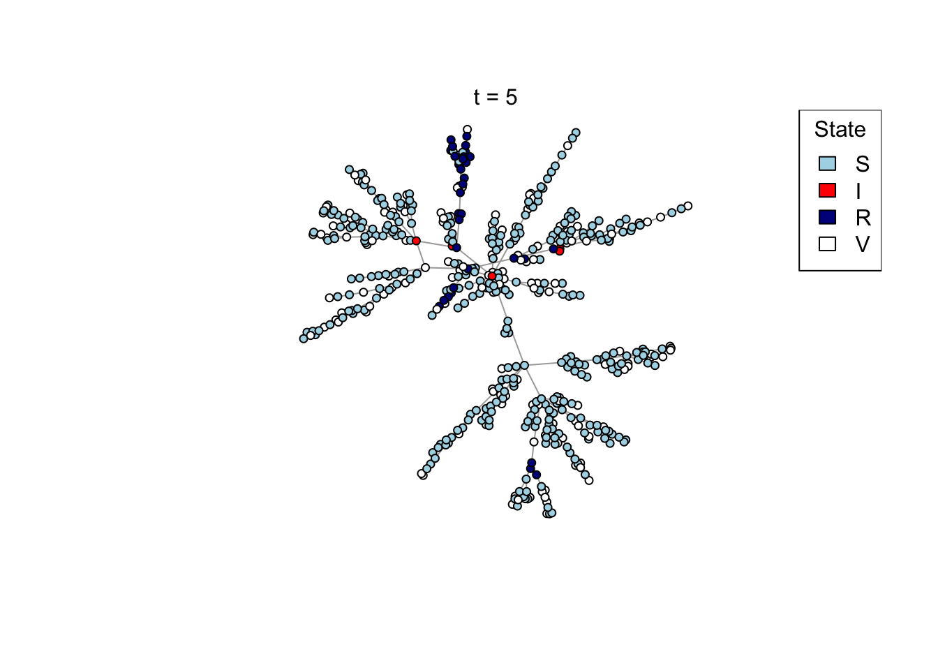
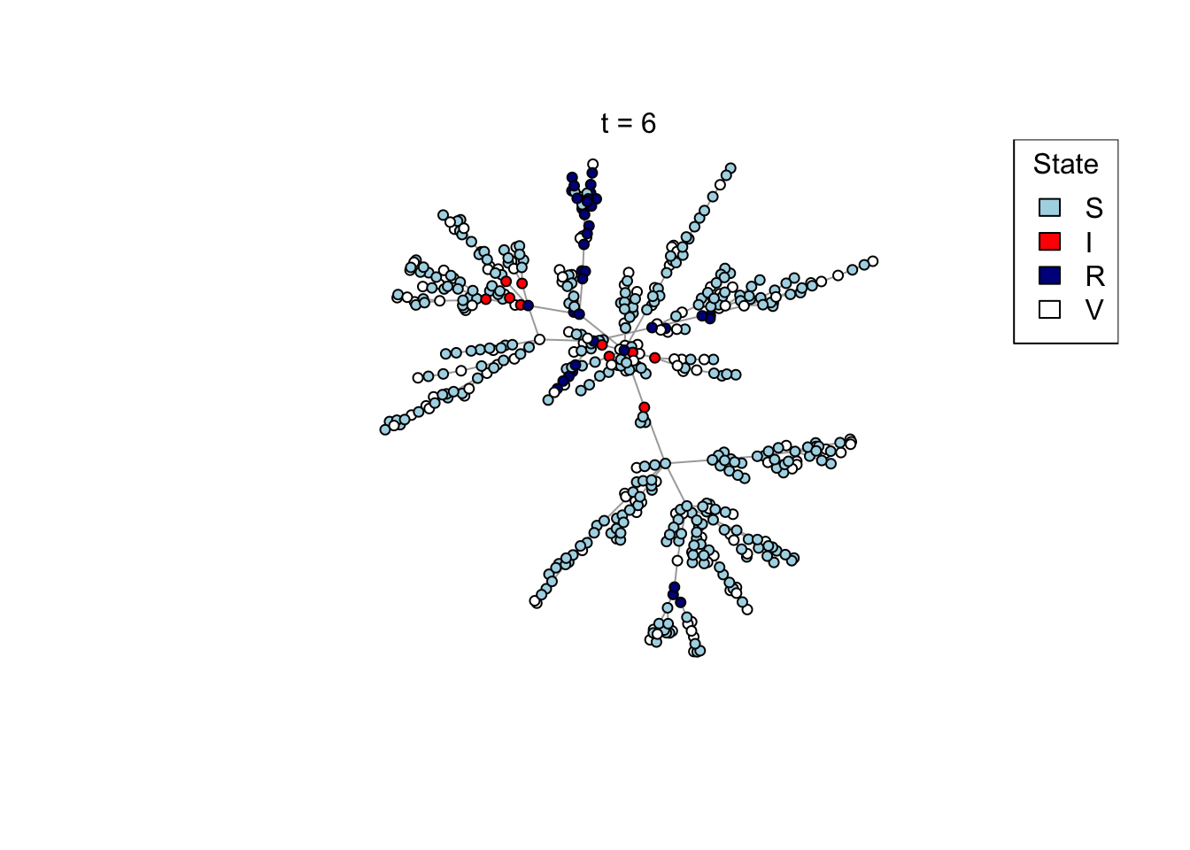
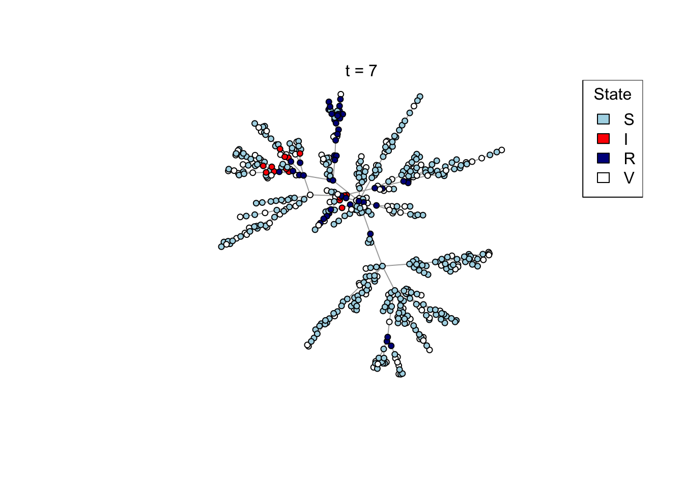
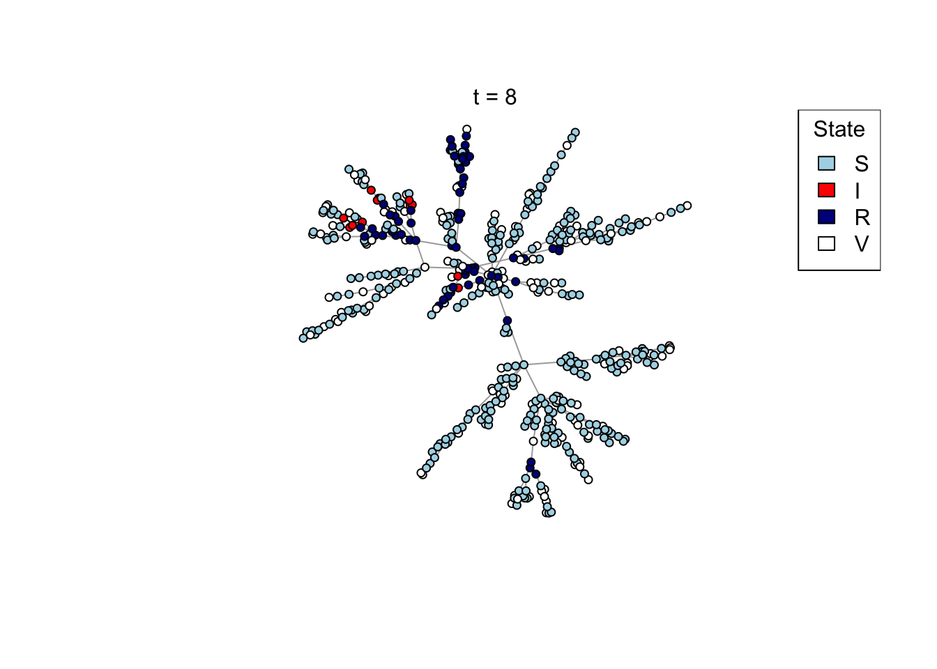
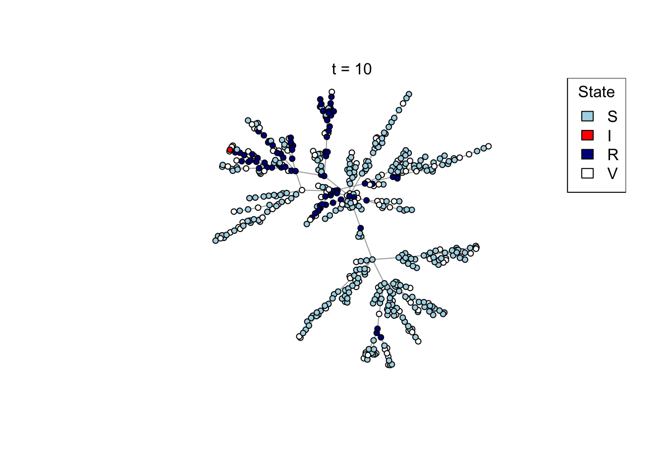
Plot a network, colouring by state (S/I/R/V).

plot_state <- function(network)
{
    # Set up palette
    colors <- c(S = "lightblue", I = "red", R = "darkblue", V = "white")
    
    # Plot network
    plot(network, 
        vertex.color = colors[V(network)$state], 
        vertex.label = NA,
        vertex.size = 4)
    legend("topright", names(colors), fill = colors, title = "State")
}

## Test the plot_state function
net <- create_network(500, 1)
plot_state(net)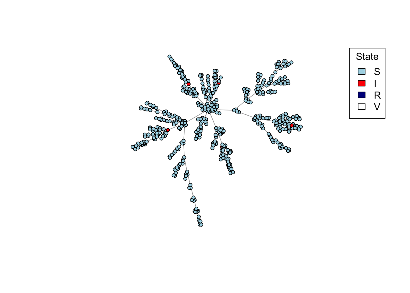

2. Running the model

Enact one step of the network model: infectious individuals infect susceptible neighbours with probability \(p\), and recover after one time step.

network_step <- function(net, p)
{
    # Identify all susceptible neighbours of infectious individuals, 
    # who are "at risk" of infection
    at_risk <- V(net)[state == "S" & .nei(state == "I")]
    
    # Use the transmission probability to select who gets exposed from
    # among those at risk
    exposed <- at_risk[runif(length(at_risk)) < p]
    
    # All currently infectious individuals will recover
    V(net)[state == "I"]$state <- "R"
    
    # All exposed individuals become infectious
    V(net)[exposed]$state <- "I"

    return (net)
}

net <- create_network(500, 1)
net <- network_step(net, p = 0.8)
plot_state(net)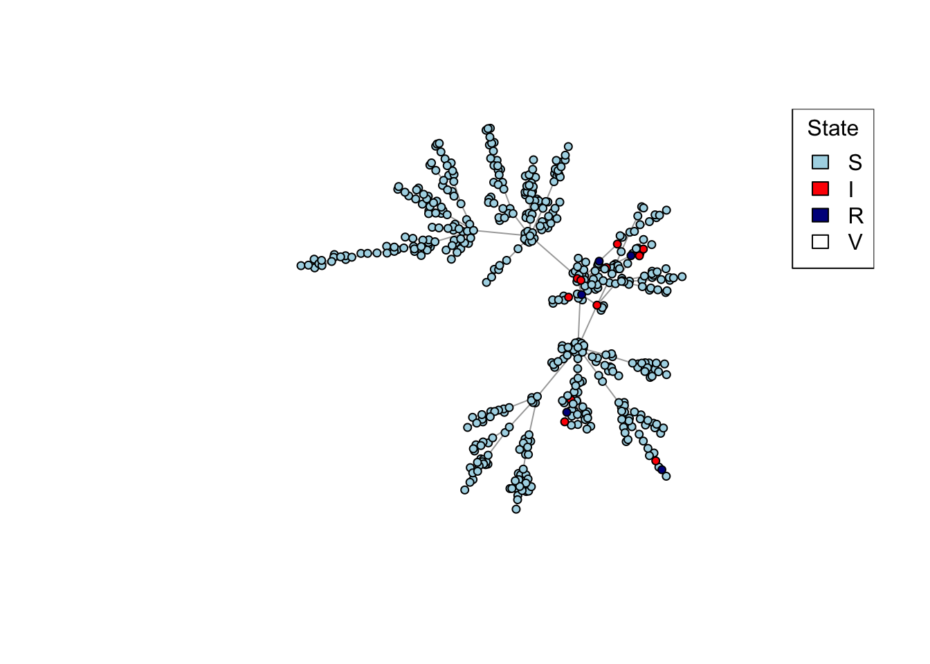

Question (3): After creating your network with the first line above, run the last two lines repeatedly to watch the network model evolve.

Run the transmission model on the network with maximum simulation time t_max
and transmission probability p; plot the network as the model is running if
animate = TRUE.

run_model <- function(net, t_max, p, animate = FALSE)
{
    # Plot network degree
    if (animate) {
        plot_degree(net)
        mtext("Network created")
        Sys.sleep(2.0)
    }

    # Set up results
    dt <- list()

    # Iterate over each time step
    for (t in 0:t_max)
    {
        # Store results
        dt[[length(dt) + 1]] <- data.table(
            S = sum(V(net)$state == "S"),
            I = sum(V(net)$state == "I"),
            R = sum(V(net)$state == "R"),
            V = sum(V(net)$state == "V")
        )

        # Plot current state
        if (animate) {
            Sys.sleep(0.5)
            plot_state(net)
            mtext(paste0("t = ", t))
        }
        
        # Stop early if no infectious individuals are left
        if (!any(V(net)$state == "I")) {
            break;
        }

        # Run one step of the network model
        net <- network_step(net, p)
    }
    
    # Return results, including empirical calculation of Rt
    results <- rbindlist(dt, idcol = "t")
    results$Rt <- results$I / shift(results$I, 1) # new infections per new infection last time step
    return (results)
}

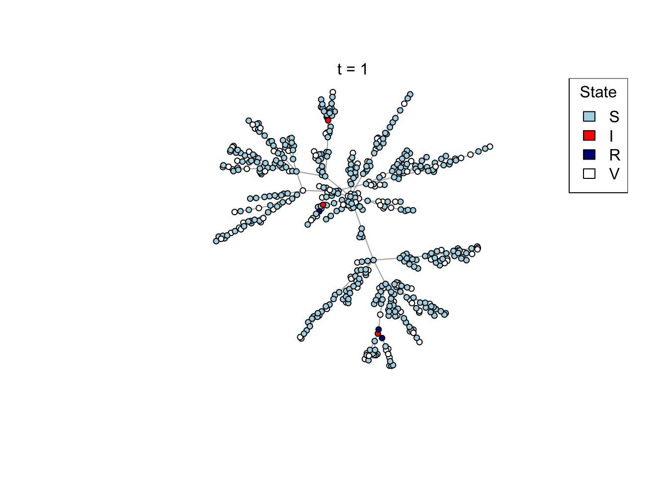
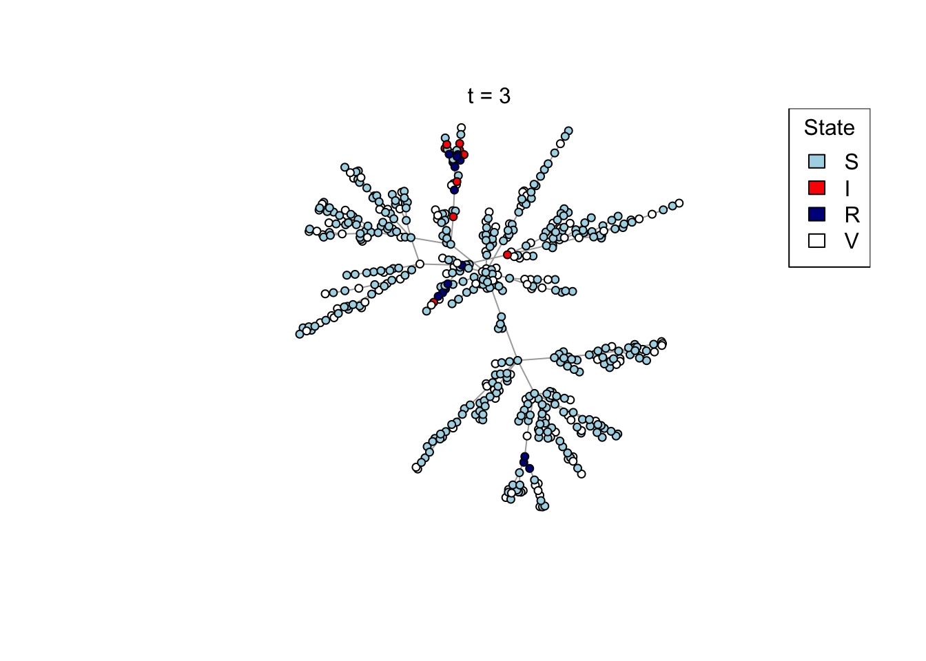
Run an example simulation

net <- create_network(500, 2)
res <- run_model(net, 100, 0.8, TRUE)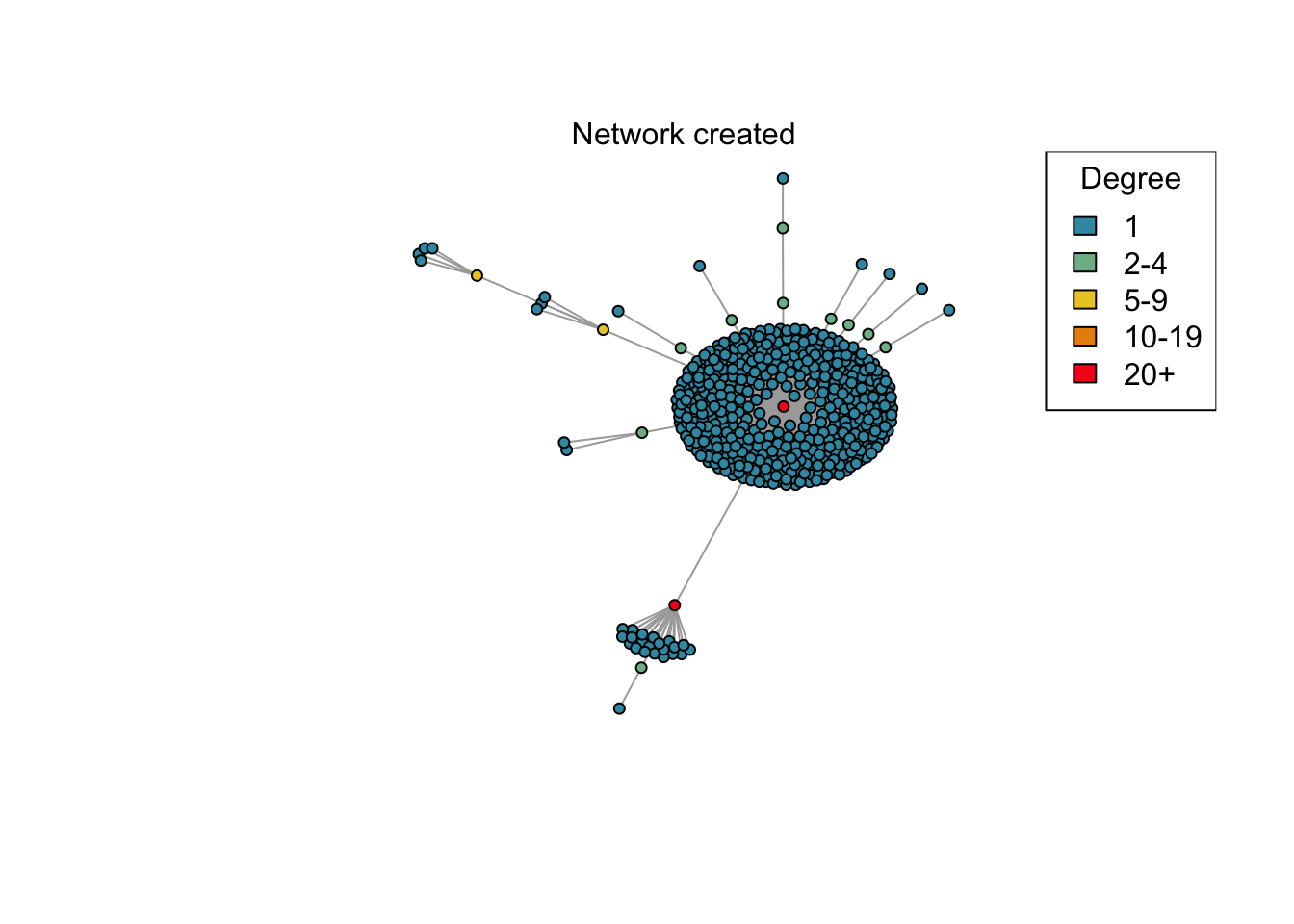

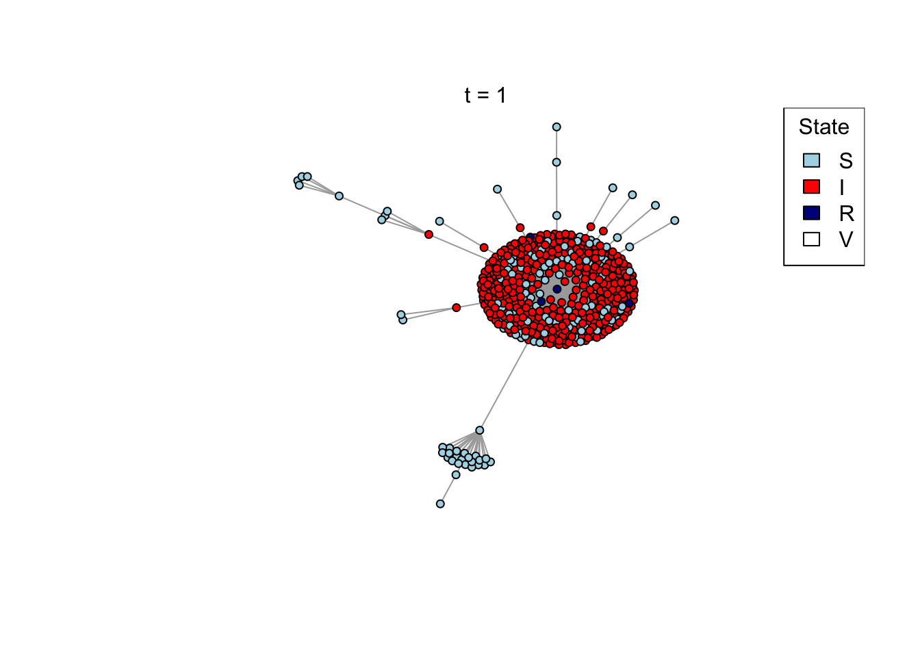
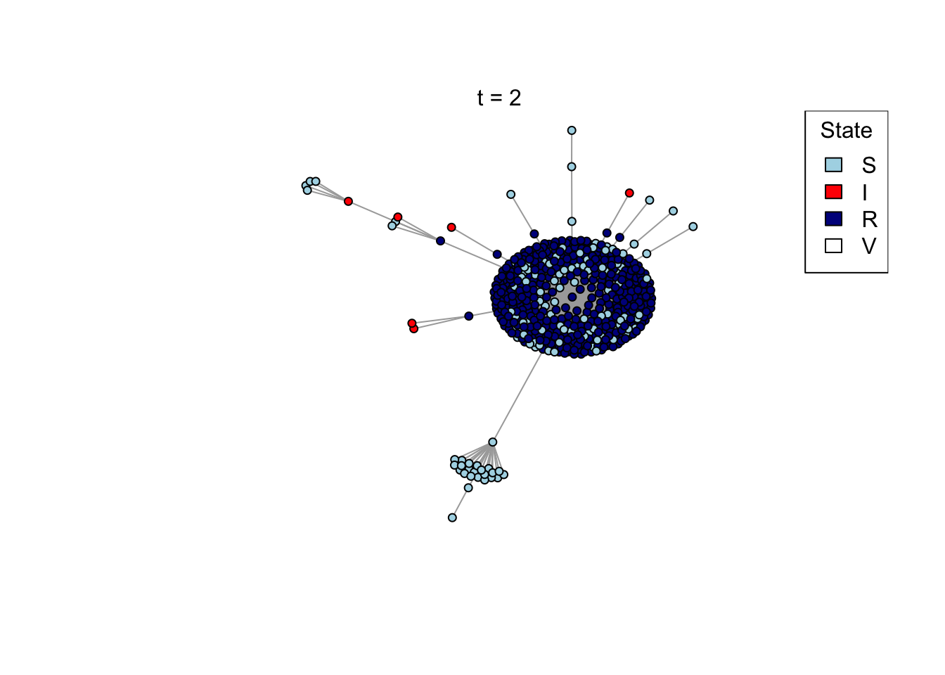
outbreak_size <- head(res$S,1) - tail(res$S,1)
print(outbreak_size)

[1] 371

Question (4): How does the preferential attachment parameter (create_network parameter d) affect the final outbreak size?

Answer: changing d from 1 to 2 increase the outbreak size, changing d from 2 to 4 doesn’t change the outbreak sizes by much.

Bonus: vaccination and multiple runs

Vaccinate a fraction v of the nodes in the network. The parameter k, between -1 and 1, determines the association between network degree and vaccination.

vaccinate_network <- function(network, v, k)
{
    # Count total population (n) and number to vaccinate (nv)
    n <- vcount(network)
    nv <- rbinom(1, n, v)

    # If k > 0, vaccinate the nv most-connected individuals; if k <= 0, 
    # vaccinate the nv least-connected individuals.
    if (k > 0) {
        target <- (n - nv + 1):n
    } else {
        target <- 1:nv
    }
    V(network)[target]$state <- "V"
    
    # Now randomly shuffle the state of a fraction 1 - abs(k) of individuals.
    shuffle <- which(rbinom(n, 1, 1 - abs(k)) == 1)
    V(network)[shuffle]$state <- sample(V(network)[shuffle]$state)

    return (network)
}

Run the model nsim times with parameters in params (n, d, v, k, t_max, p), showing the animated network the first nanim times, and returning a data.table with the results of each simulation.

run_scenario <- function(params, nsim, nanim = 1)
{
    results <- list()
    
    for (sim in 1:nsim)
    {
        net <- create_network(params$n, params$d)
        net <- vaccinate_network(net, params$v, params$k)

        results[[sim]] <- run_model(net, params$t_max, params$p, animate = sim <= nanim)
        
        cat(".")
    }
    cat("\n");
    
    results <- rbindlist(results, idcol = "run")
    return (results)
}

Test multiple runs

params <- list(
    n = 500,
    d = 0,
    p = 0.8,
    v = 0.3,
    k = -0.5,
    t_max = 100
)

# Do a test run!
x <- run_scenario(params, nsim = 50)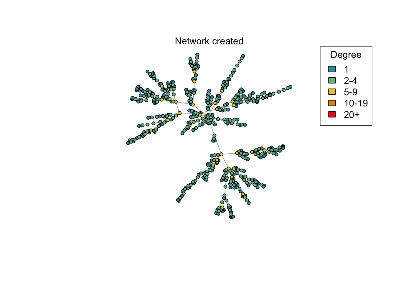

..................................................

ggplot(x) +
    geom_line(aes(x = t, y = R, group = run))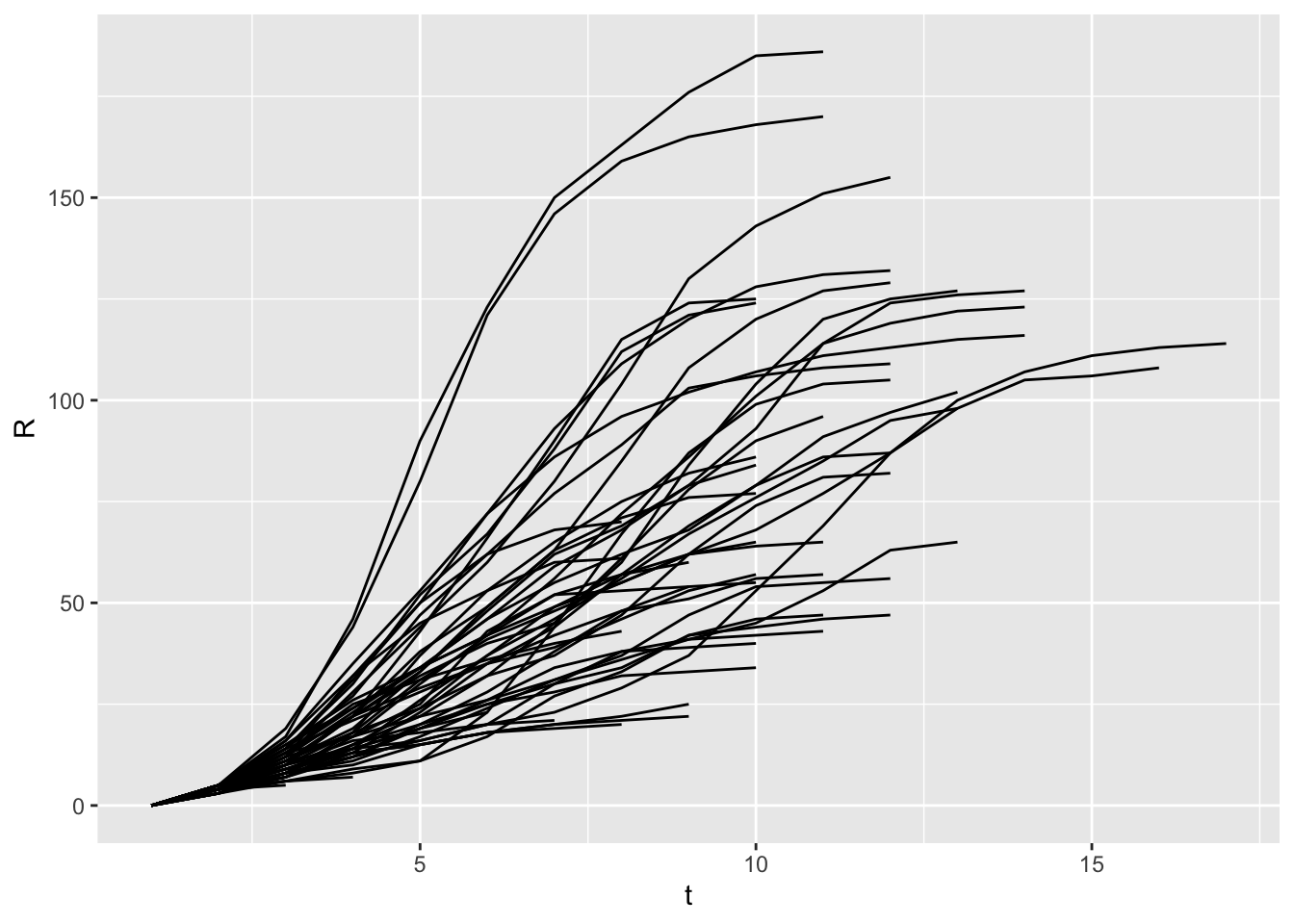

Return to the practical here.