Example 1: Mixture model

David Hodgson

2024-12-22

This markdown block outlines a simulation study designed to demonstrate how RJMCMC can be used to recover the parameters of a mixture model. Here’s what it does:

• Purpose: Highlight the ability of RJMCMC to estimate parameters and select the number of components in a mixture model.
• Steps: Systematically define the target distribution, simulate data, apply RJMCMC, and analyze the results.
• RJMCMC Role: It enables the model to explore variable-dimensional parameter spaces (different $K$) while estimating component parameters $(\mu_k, \sigma_k, \pi_k)$.

This block serves as a guide for implementing and understanding RJMCMC in the context of mixture model recovery. If you’d like, I can help add technical details or coding snippets to complement it!

Link to methods

1. Relevant packages

library(devtools)
devtools::load_all()
library(lubridate)
library(patchwork)
library(tidybayes)
library(ggdist)

# Using more than one core might fail on windows, 
if (.Platform$OS.type == "windows") {
  mc.cores <- 1
} else {
  mc.cores <- 2 # use as many as available, preferably 4.
}

2. Simulated data

We aim to recover the parameters of a mixture distribution using Reversible Jump Markov Chain Monte Carlo (RJMCMC). The target mixture distribution is defined as follows:

• Mixture of $K$ Gaussian components.
• Each component has:
  • Mean ($\mu_k$).
  • Standard deviation ($\sigma_k$).
  • Mixing proportion ($\pi_k$).

• 2.1 Key Parameters

1. $K$: Number of Components
   • Inferred during the RJMCMC process.
   • Represented indirectly as the number of columns in the jump matrix.
   • Birth and death proposals dynamically add or remove components.
2. $\sigma$: Standard Deviation
   • Represents the standard deviation for each Gaussian component.
   • Sampled and updated during the RJMCMC steps.
   • Plays a role in the likelihood evaluation through dnorm.
3. $\mu$: Mean
   • Represents the mean of each Gaussian component.
   • Sampled and updated during the RJMCMC steps.
   • Guides the location of the mixture components.
4. $p$: Mixing Proportions
   • Determines the weight of each Gaussian component in the mixture.
   • Constrained to sum to 1, handled during proposals (e.g., sampleBirthProposal).

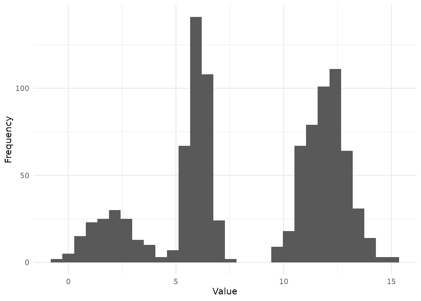
Therefore, we simulate a dataset from a predefined mixture model with known parameters ($K, \mu_k, \sigma_k, \pi_k$). Here,

• K = 3
• $\mu_k$ = 2, 6, 12
• $\sigma_k$ = 1, 0.5, 1
• $\pi_k$ = 0.3, 0.7, 1

m <- 5
# Run the model 
obs <- c(sample(rnorm(10e4, 2, 1), 30 * m, replace = TRUE),
    sample(rnorm(10e4, 6, 0.5), 70 * m, replace = TRUE), 
    sample(rnorm(10e4, 12, 1), 100 * m, replace = TRUE))


library(ggplot2)
ggplot() + geom_histogram(aes(obs), bins = 30) + theme_minimal() + labs(x = "Value", y = "Frequency")

3. Simulation recovery

3.1 Description of the model

The model represents a Gaussian mixture distribution with the following key components:

1. Mixture Structure:
   • The distribution is a combination of multiple Gaussian components.
   • Each component is defined by its:
     • Mean ($\mu_k$).
     • Standard deviation ($\sigma_k$).
     • Mixing proportion ($p_k$).
2. Mathematical Representation:
   • The probability density function for an observation $z$ is given by: $$p(z) = \sum_{k=1}^K p_k \cdot \mathcal{N}(z \mid \mu_k, \sigma_k^2)$$ where:
     • $\mathcal{N}(z \mid \mu_k, \sigma_k^2)$ is the normal density for the $k$-th component.
     • $p_k$ represents the mixing proportion of the $k$-th component.
     • $K$ is the number of components.
3. Parameters to Infer:
   • $K$: The number of mixture components, which is inferred dynamically using RJMCMC.
   • $p_k$: Mixing proportions, constrained such that $\sum_{k=1}^K p_k = 1$.
   • $\mu_k$: Means of the components, defining their location.
   • $\sigma_k$: Standard deviations, defining their spread.
4. Dynamic Nature of the Model:
   • The number of components ($K$) is not fixed and can change as the algorithm proposes and evaluates birth or death moves.
   • This allows the model to adaptively determine the most probable number of components based on the observed data.
5. Likelihood Function:
   • The likelihood of the data given the parameters is: $$\mathcal{L}(\text{data} \mid K, \{p_k, \mu_k, \sigma_k\}) = \prod_{i=1}^N \left( \sum_{k=1}^K p_k \cdot \mathcal{N}(z_i \mid \mu_k, \sigma_k^2) \right)$$ where $N$ is the total number of data points.
6. Prior Assumptions:
   • $p_k$: Uniform distribution over the simplex.
   • $\mu_k$: Uniform distribution over a predefined range (e.g., [0, 20]).
   • $\sigma_k$: Uniform distribution over a positive range (e.g., [0.3, 3]).
   • $K$: Uniform prior over a predefined integer range (e.g., [1, 8]).

This model structure allows the RJMCMC algorithm to infer both the number of components and their parameters, effectively capturing the complexity of the underlying data distribution.

3.2 Steps to Recover $(K, \mu, p, \sigma)$:

1. Initialization Functions

• sampleInitPrior:
  • Samples the initial value for the parameter (e.g., $\sigma$).
• sampleInitJump:
  • Initializes the jump matrix, representing the mixture parameters:
    • First row: mixing proportions $p$.
    • Second row: means $\mu$.
    • Third row: standard deviations $\sigma$.

2. Prior and Likelihood Evaluations

• evaluateLogPrior:
  • Computes the log-prior probability for all parameters.
  • Ensures parameters like $p, \mu, \sigma$ are within their respective bounds.
  • Includes a uniform prior for the number of components ($K$).
• evaluateLogLikelihood:
  • Computes the log-likelihood of the data given the current parameter values.
  • Uses the Gaussian mixture model equation: $$L = \sum_{i=1}^{N_{\text{data}}} \log\left(\sum_{j=1}^K p_j \cdot \mathcal{N}(z_i \mid \mu_j, \sigma_j)\right)$$ where $z$ is the observed data.

3. Birth and Death Proposals

• sampleBirthProposal:
  • Adds a new component by sampling:
    • $p$: a new mixing proportion.
    • $\mu$: a new mean.
    • $\sigma$: a new standard deviation.
  • Adjusts existing $p$ values to ensure they sum to 1.
• sampleDeathProposal:
  • Removes a randomly selected component.
  • Adjusts the remaining $p$ values to maintain normalization.
• evaluateBirthProposal:
  • Evaluates the probability of proposing a new component.
• evaluateDeathProposal:
  • Evaluates the probability of proposing to remove a component.

4. Jump and Proposal Sampling

• sampleJump:
  • Updates the parameters of a specific component:
    • Adjusts $p, \mu, \sigma$ for the selected component.
    • Introduces small random changes.
• sampleProposal:
  • Decides whether to perform a birth, death, or jump move.
  • Probabilities vary depending on the current number of components.

Overall Process in RJMCMC

1. Initialization:
   • Start with initial values for $\sigma$ and the jump matrix.
2. Proposal Steps:
   • Select a move type (birth, death, or jump) based on sampleProposal.
   • Apply the corresponding function (e.g., sampleBirthProposal).
3. Evaluation:
   • Compute the prior and likelihood for the proposed parameters.
   • Use the Metropolis-Hastings acceptance rule to decide whether to accept or reject the proposal.
4. Iteration:
   • Repeat steps to explore the posterior distribution of $K$, $\sigma$, $\mu$, and $p$.

---

model <- list(

  lowerParSupport_fitted = c(-8),
  upperParSupport_fitted = c(8),

  namesOfParameters = c("sigma"),

  sampleInitPrior = function(datalist) {
    rnorm(1, 0, 1)
  },

  sampleInitJump = function(params, datalist) {
    p <- c(0.5, 0.5)
    mu <- c(1, 4)
    sigma <- c(1, 1)
    jump_new <- matrix(c(p, mu, sigma), nrow = 3, byrow = TRUE)
    jump_new
  },

  evaluateLogPrior = function(params, jump, datalist) {
    p <- dnorm(params[1], 0, 1, log = TRUE)

    p_vec <- jump[1, ]
    for(i in 1:length(p_vec) ) {
        p <- p + dunif(p_vec[i], 0, 1, log = TRUE)
    }
    mu_vec <- jump[2, ]
    for(i in 1:length(mu_vec) ) {
        p <- p + dunif(mu_vec[i], 0, 20, log = TRUE)
    }
    sigma_vec <- jump[3, ]
    for(i in 1:length(sigma_vec) ) {
        p <- p + dunif(sigma_vec[i], 0.3, 3, log = TRUE)
    }
    N <- ncol(jump)
    p <- p + dunif(N, 1, 8)

  #  cat("prior: ", str(p))
    p
  },

  evaluateLogLikelihood = function(params, jump, datalist) {
   # cat("in:  evaluateLogLikelihood")
    ll <- 0
    N <- ncol(jump)
    p_vec <- jump[1, ]

    mu_vec <- jump[2, ]
    sigma_vec <- jump[3, ]

    z <- datalist$obs
    N_data <- datalist$N_data
    sigma <- params[1]

    for (i in 1:N_data) {
        i_x = 0
        for (j in 1:N) {
            i_x <- i_x + p_vec[j] * dnorm(z[i], mu_vec[j], sigma_vec[j])
        }
        ll <- ll + log(i_x)
    }

   # cat("loglik: ", str(ll) )
    ll
  },

  sampleBirthProposal =  function(params, jump, i_idx, datalist) {
    p_new_sample <- runif(1, 0, 1)
    p_new <- c(jump[1, ] * (1 - p_new_sample), p_new_sample)
    mu_new_sample <- runif(1, 0, 20)
    mu_new <- c(jump[2, ], mu_new_sample)
    sigma_new_sample <- runif(1, 0.3, 3)
    sigma_new <- c(jump[3, ], sigma_new_sample)
    jump_new <- matrix(c(p_new, mu_new, sigma_new), nrow = 3, byrow = TRUE)
    jump_new
  },

  sampleDeathProposal = function(params, jump, i_idx, datalist) {

    N <- ncol(jump)
    jump_remove <- jump[, i_idx]
    jump_new <- jump[, -i_idx]
    jump_new[1, ] <- c(jump_new[1, ] / (1 - jump_remove[1]))
    jump_new
  },

  evaluateBirthProposal = function(params, jump, i_idx, datalist) {

    N <- ncol(jump)
    log(1 / (N * dunif(jump[2, N], 0, 20 ) ))
  },

  evaluateDeathProposal = function(params, jump, i_idx, datalist) {

    N <- ncol(jump)
    log((N) * dunif(jump[2, i_idx], 0, 20 ) ) 
  },

  sampleJump = function(params, jump, i_idx, datalist) {

    N <- ncol(jump)
    jump_update <- jump[, i_idx]

    p_new <- min(max(jump_update[1] + rnorm(1, 0, 0.01), 0), 1)
    diff = (jump_update[1] - p_new) / (N - 1)
    p_new_vew <- jump[1, ] + diff
    p_new_vew[i_idx] <- p_new
    jump[1, ] <- p_new_vew

    jump[2, i_idx] <- jump_update[2] + rnorm(1, 0, 0.1)
    jump[3, i_idx] <- max(jump_update[3] + rnorm(1, 0, 0.1), 0.3)

    jump
  },

  sampleProposal = function(params, jump, datalist) {
    N <- ncol(jump)
    if (N == 2) {
      q <- c(0.0, 0.67, 1.0)
    } else if (N == 20) {
      q <- c(0.33, 1.0, 1.0)
    } else {
      q <- c(0.33, 0.67, 1.0)
    }
    q
  }

)

3.3. Settings and run model

This code block defines the settings for the RJMCMC algorithm, prepares the input data, executes the model, and saves the results. Below is a breakdown of its components:

1. Define Settings

The settings list specifies the configuration for the RJMCMC run:

• numberChainRuns: Specifies the number of independent MCMC chains to run (e.g., 4 chains).
• numberCores: Indicates the number of CPU cores allocated for computation. Parallel processing is possible if runParallel = TRUE.
• iterations: Sets the total number of iterations for each MCMC chain (e.g., 4000 iterations).
• burninPosterior: Defines the number of initial iterations to discard as burn-in (e.g., 2000 iterations).
• thin: Thinning interval to reduce autocorrelation by retaining only every $n$-th sample (e.g., every 10th sample).
• runParallel: Boolean flag controlling whether chains are run in parallel (FALSE here indicates sequential execution).
• onDebug: Boolean flag for enabling debugging mode, which can output additional information during execution.

---

2. Prepare Data

The data_l list structures the observed data for use in the RJMCMC function: - obs: A vector containing the observed data points, likely representing samples drawn from an unknown mixture distribution. - N_data: The total number of observations, calculated as the length of the obs vector.

This organized format ensures compatibility with the rjmc_func function.

---

3. Run the Model

The rjmc_func function executes the RJMCMC algorithm using: - model: The previously defined RJMCMC model, containing prior distributions, likelihood functions, and proposal mechanisms. - data_l: The structured data list, providing the observed values and their count. - settings: The configuration for the MCMC run.

The output, stored in the outputs object, contains the results of the RJMCMC process, including posterior samples and diagnostics for the model parameters.

---

# Define the settings
settings <-  list(
    numberCores = mc.cores,
    numberChainRuns = 4,
    iterations = 10000,
    burninPosterior = 5000,
    thin = 10
)

data_l <- list(
    obs = obs,
    N_data = length(obs)
)

outputs <- rjmc_func(model, data_l, settings)
saveRDS(outputs, here::here("outputs", "fits", "mixture_norm", "fit_sim_null.RDS"))

4. Analyse the posterior distributions

This section examines the posterior distributions generated by the RJMCMC algorithm. We aim to evaluate the ability of the model to recover key parameters of the mixture distribution, such as the number of components ($K$), the mixing proportions ($p$), the means ($\mu$), and the standard deviations ($\sigma$).

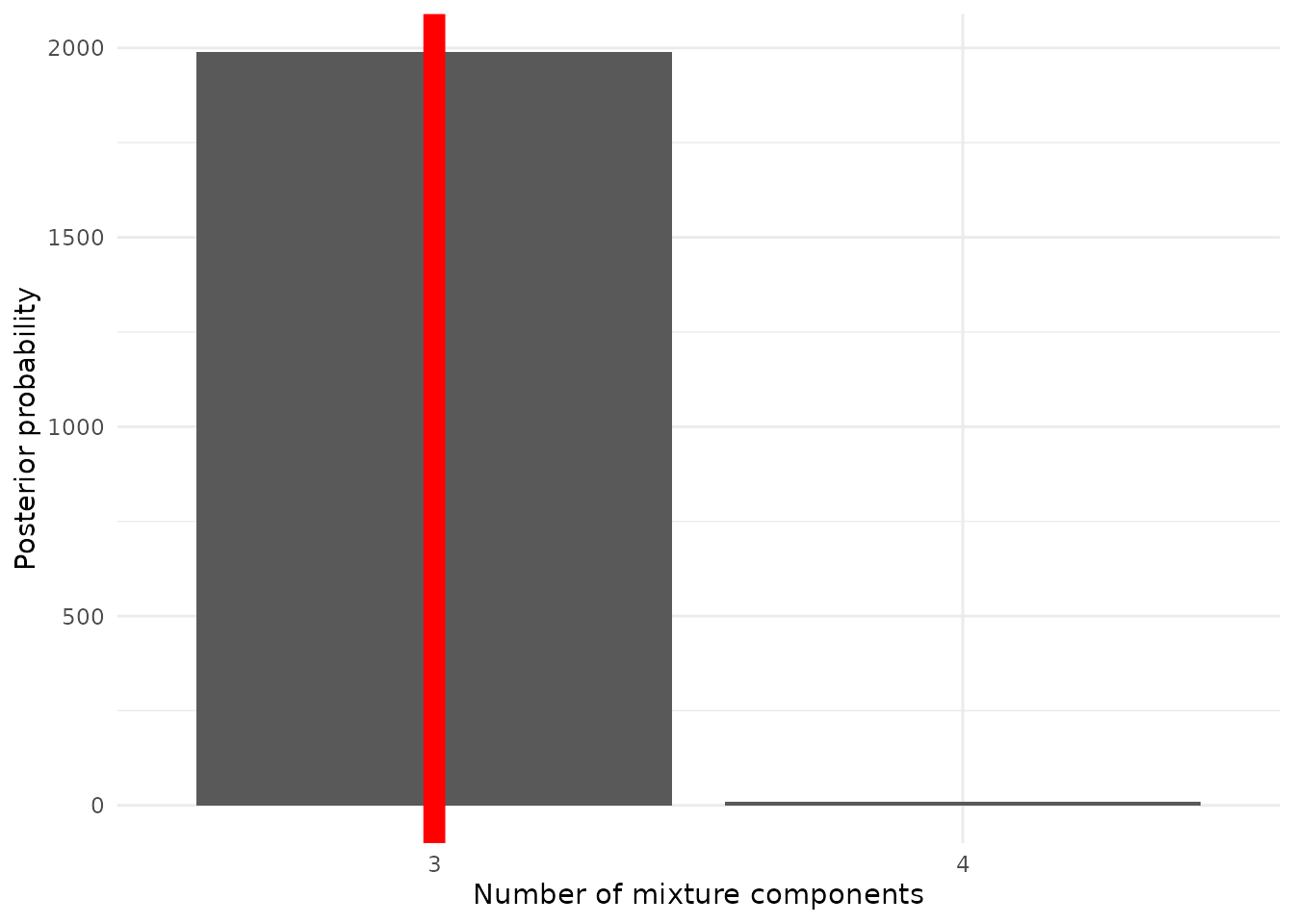
4.1 Simulation recovery of K

In this subsection, we analyze the posterior distribution of the number of mixture components ($K$). The posterior probabilities for different values of $K$ are calculated, and the mode of the posterior distribution is compared to the true value. The bar chart below illustrates the posterior probabilities for the number of components, with the true value highlighted by a red vertical line:

require(patchwork)
require(purrr)
require(ggplot2)

n_chain <- 4

tables_length <- get_lengths(outputs, n_chain)

df_K_post <- data.frame(
  dim = names(tables_length),
  post = as.vector(tables_length)
)

df_K_post %>% ggplot() + 
  geom_col(aes(x = dim, y = post)) + theme_minimal() + 
  geom_vline(xintercept = c("3"), color = "red", size = 4) +
  labs(x = "Number of mixture components", y = "Posterior probability")

4.2 Simulation recovery of p, mu, sigma

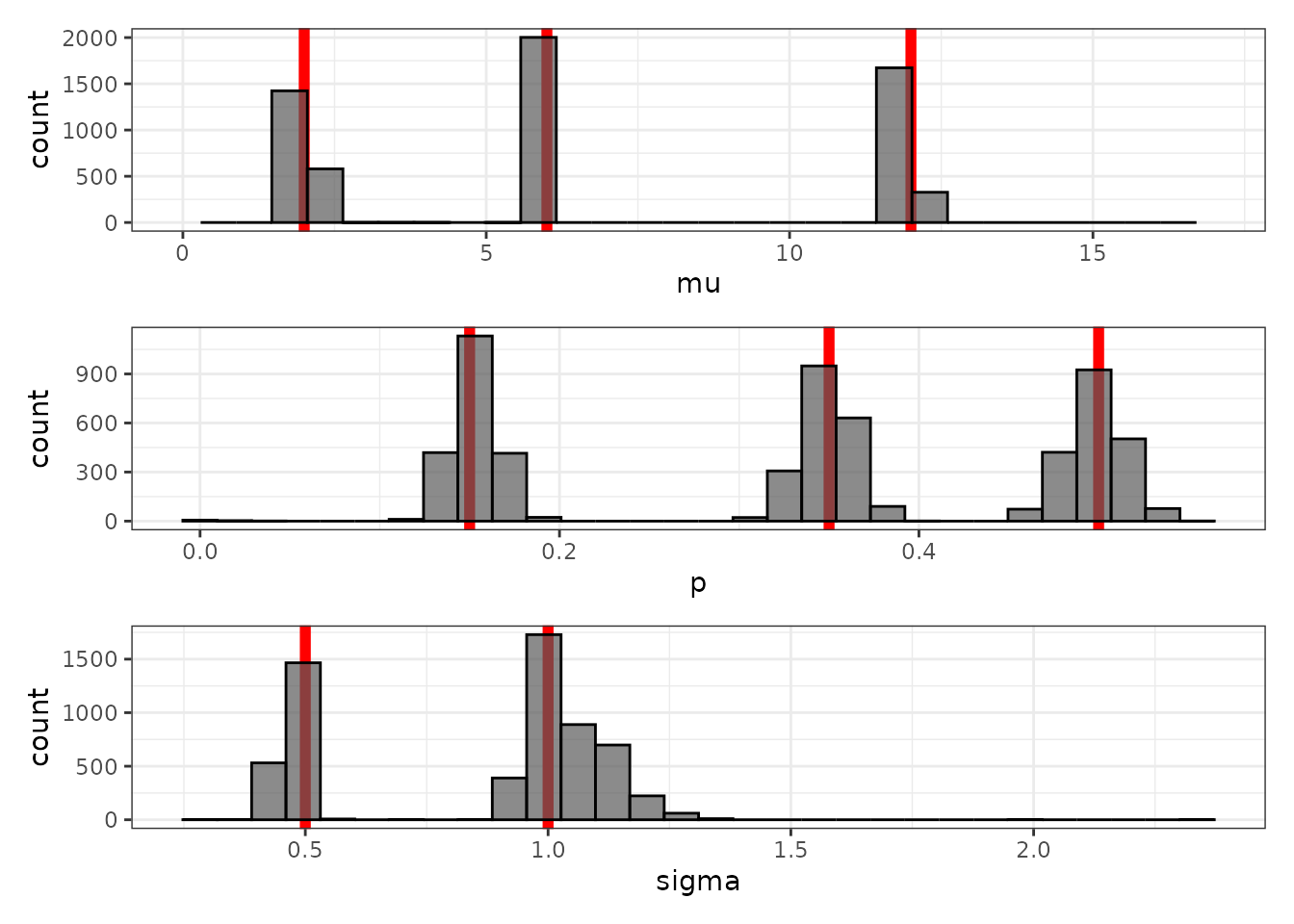
Here, we examine the posterior distributions of the mixing proportions (p), means (μ), and standard deviations (σ) for the mixture components. Histograms are used to visualize the posterior samples, with the true values highlighted by red vertical lines.

The histograms provide insights into the precision of the RJMCMC algorithm in recovering the true parameter values.

posterior_sample <- map_df(1:4, 
  function(y) {
    map_df(1:length(outputs$jump[[y]]), 
      function(x) {
        outputs$jump[[y]][[x]] %>% t %>% as.data.frame %>% arrange(V2) %>% mutate(n = 1:nrow(.), sample = x, chain = y) %>%
          set_names(c("p", "mu", "sigma", "n", "sample", "chain")) %>% pivot_longer(-c(n, sample, chain), names_to = "parameter", values_to = "values" )
      }
    )
  }
) %>% pivot_wider(names_from = "parameter", values_from = "values") 

p1 <- posterior_sample %>% ggplot() +    
  geom_vline(xintercept = c(2, 6, 12), color = "red", size = 2) +
  geom_histogram(aes(mu), color = "black", alpha = 0.7) + theme_bw() + 
  xlim(0, 17)

p2 <- posterior_sample %>% ggplot() +    
  geom_vline(xintercept = c(0.15, 0.35, 0.5), color = "red", size = 2) +
  geom_histogram(aes(p), color = "black", alpha = 0.7) + theme_bw()


p3 <- posterior_sample %>% ggplot() +    
  geom_vline(xintercept = c(1, 0.5, 1 ), color = "red", size = 2) +
  geom_histogram(aes(sigma), color = "black", alpha = 0.7) + theme_bw()

p1 / p2 / p3

4.3 Summary of the posterior distributions

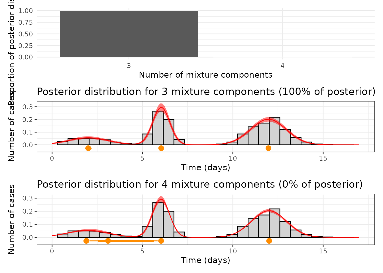
This subsection summarizes the posterior distributions of the mixture model, focusing on the most probable number of components (K) and the associated parameter values. The posterior proportions for each K are calculated, and the posterior trajectory of parameters is visualized for selected values of K.

The first plot below shows the posterior proportions for the number of components (K). Subsequent plots visualize the posterior trajectories for p, μ, and σ for K = 3 and K = 4.

tables_length <- get_lengths(outputs, n_chain)

mode_post <- names(sort(tables_length, decreasing = TRUE))[1]
mix_size <- mode_post

post_process_3 <- get_clean_posterior(outputs, "3", 4)
post_process_4 <- get_clean_posterior(outputs, "4", 4)

prop <- tables_length / sum(tables_length)
plotl <- prop[mix_size]

p0 <- ggplot() + geom_col(aes(x = names(prop), y = prop)) + ylim(0, 1) + theme_minimal() + 
  labs(x = "Number of mixture components", y = "Proportion of posterior distribution")

p1_anot <- get_posterior_component_size("3", tables_length, post_process_3, data_l)
p2_anot <- get_posterior_component_size("4", tables_length, post_process_4, data_l)

p0 / p1_anot / p2_anot

This analysis highlights the posterior support for different numbers of components and provides a detailed summary of the recovered parameters for the most probable configurations.