######################################################
#              ODEs in R: Practical 2                #
######################################################

# Load in the deSolve package
library(deSolve)
# If the package is not installed, install using the install.packages() function

########## PART I. TIME DEPENDENT TRANSMISSION RATE

# The code below is for an SI model with a time dependent transmission rate.
# The transmission rate is a function of the maximum value of beta (beta_max)
# and the period of the cycle in days.

# Define model function
SI_seasonal_model <- function(t, state, parms)
{
    # Get variables
    S <- state["S"]
    I <- state["I"]
    N <- S + I
    # Get parameters
    beta_max <- parms["beta_max"]
    period <- parms["period"]
    # Calculate time-dependent transmission rate
    beta <- beta_max / 2 * (1 + sin(2*pi*t / period))
    # Define differential equations
    dS <- -(beta * S * I) / N
    dI <- (beta * S * I) / N
    res <- list(c(dS, dI))
    return (res)
}

# Define parameter values
parameters <- c(beta_max = 0.4, period = 10)

# Define time to solve equations
times <- seq(from = 0, to = 50, by = 1)

# 1. Plot the equation of beta against a vector of times to understand the time
#    dependent pattern.
# How many days does it take to complete a full cycle?
# How does this relate to the period?

# Extract parameters
beta_max <- parameters["beta_max"]
period <- parameters["period"]
# Calculate time dependent transmission rate
beta <- beta_max / 2 * (1 + sin(times * (2 * pi / period) ) )

plot(times, beta, type = "l")

# Answer: 10 days; this is the period.

# 2. Now solve the model using the function ode and plot the output
# HINT: you need to write the state vector and use the ode function
# using func = SI_seasonal_model

# Define initial conditions
N <- 100
I_0 <- 1
S_0 <- N - I_0
state <- c( S = S_0, I = I_0)

# Solve equations
output_raw <- ode(y = state, times = times, func = SI_seasonal_model, parms = parameters)
# Convert to data frame for easy extraction of columns
output <- as.data.frame(output_raw)

# Plot output
par(mfrow = c(1, 1))
plot(output$time, output$S, type = "l", col = "blue", lwd = 2, ylim = c(0, N),
      xlab = "Time", ylab = "Number")
lines(output$time, output$I, lwd = 2, col = "red")
legend("topright", legend = c("Susceptible", "Infected"),
       lty = 1, col = c("blue", "red"), lwd = 2, bty = "n")

# 3. Change the period to 50 days and plot the output. What does the model output look like?
# Can you explain why?

# Change parameters
parameters["period"] <- 50

# Run ODEs again
output_raw <- ode(y = state, times = times, func = SI_seasonal_model, parms = parameters)
output <- as.data.frame(output_raw)

# Plot output
par(mfrow = c(1, 1))
plot(output$time, output$S, type = "l", col = "blue", lwd = 2, ylim = c(0, N),
      xlab = "Time", ylab = "Number")
lines(output$time, output$I, lwd = 2, col = "red")
legend("topright", legend = c("Susceptible", "Infected"),
       lty = 1, col = c("blue", "red"), lwd = 2, bty = "n")

# Answer:
# The period is longer than the vector of times, so a full cycle is not completed within
# our model solution


########## PART II. USING EVENTS IN DESOLVE

## deSolve can also be used to include 'events'. 'events' are triggered by
# some specified change in the system.

# For example, assume an SI model with births represents infection in a livestock popuation.
# If more than half of the target herd size becomes infected, the infected animals are culled
# at a daily rate of 0.5.

# As we are using an open population model (i.e. a model with births and/or deaths),
# we have two additional parameters governing births: the birth rate b, and the
# target herd size (or carrying capacity), K

# Define model function
SI_open_model <- function(times, state, parms)
{
    ## Define variables
    S <- state["S"]
    I <- state["I"]
    N <- S + I
    # Extract parameters
    beta <- parms["beta"]
    K <- parms["K"]
    b <- parms["b"]
    # Define differential equations
    dS <- b * N * (K - N) / K - (beta * S * I) / N
    dI <- (beta * S * I) / N
    res <- list(c(dS, dI))
    return (res)
}

# Define time to solve equations
times <- seq(from = 0, to = 100, by = 1)

# Define initial conditions
N <- 100
I_0 <- 1
S_0 <- N - I_0
state <- c(S = S_0, I = I_0)

# 4. Using beta = 0 (no infection risk), K = 100, b = 0.1, and an entirely susceptible
# population (I_0 = 0), investigate how the population grows with S_0 = 1, 50 and 100.

# What size does the population grow to? Why is this?
# Answer: 100 always, this is due to the managed births via the target herd size.

# How do you increase this threshold?
# Answer: Increase the parameter K.

# Define parameter values
# K is our target herd size, b is the birth rate)
parameters <- c(beta = 0, K = 100, b = 0.1)

# To include an event we need to specify two functions:
# the root function, and the event function.

# The root function is used to trigger the event
root <- function(times, state, parms)
{
    # Get variables
    S <- state["S"]
    I <- state["I"]
    N <- S + I
    # Get parameters
    K <- parms["K"]
    # Our condition: more than half of the target herd size becomes infected
    # We want our indicator to cross zero when this happens
    indicator <- I - K * 0.5
    return (indicator)
}

# The event function describes what happens if the event is triggered
event_I_cull <- function(times, state, parms)
{
    # Get variables
    I <- state["I"]

    # Extract parameters
    tau <- parms["tau"]

    I <- I * (1 - tau) # Cull the infected population

    state["I"] <- I # Record new value of I

    return (state)
}

# We add the culling rate tau to our parameter vector
parameters <- c(beta = 0.1, K = 100, tau = 0.5, b = 0.1)

# Solve equations
output_raw <- ode(y = state, times = times, func = SI_open_model, parms = parameters,
                  events = list(func = event_I_cull, root = TRUE), rootfun = root)
# Convert to data frame for easy extraction of columns
output <- as.data.frame(output_raw)

# Plot output
par(mfrow = c(1, 1))
plot(output$time, output$S, type = "l", col = "blue", lwd = 2, ylim = c(0, N),
     xlab = "Time", ylab = "Number")
lines(output$time, output$I, lwd = 2, col = "red")
legend("topright", legend = c("Susceptible", "Infected"),
       lty = 1, col = c("blue", "red"), lwd = 2, bty = "n")

# 5. What happens to the infection dynamics when the infected animals are culled?

# Answer: the herd is culled when more than 50% of the target herd size is infected
# but this is not enough to eradicate infection in the population. The infected herd
# size goes back up to 50% and is culled again, this cycle continues.


# 6. Assume now that when an infected herd is culled, the same proportion of
# animals is ADDED to the susceptible population.

# HINT: you will need to change the event function to include additions to the
# S state.

event_SI_cull <- function(times, state, parms)
{
    # Get variables
    S <- state["S"]
    I <- state["I"]

    # Get parameters
    tau <- parms["tau"]

    S <- S * (1 + tau) # replenish the susceptible population
    I <- I * (1 - tau) # cull the infected population

    state["S"] <- S
    state["I"] <- I

    return (state)
}

# 7. What happens to the infection dynamics when the infected animals are culled?
# How is this different to when only infected animals are culled?

# Solve equations
output_raw <- ode(y = state, times = times, func = SI_open_model, parms = parameters,
                  events = list(func = event_SI_cull, root = TRUE), rootfun = root)
# Convert to data frame for easy extraction of columns
output <- as.data.frame(output_raw)

# Plot output
par(mfrow = c(1, 1))
plot(output$time, output$S, type = "l", col = "blue", lwd = 2, ylim = c(0, N),
     xlab = "Time", ylab = "Number")
lines(output$time, output$I, lwd = 2, col = "red")
legend("topright", legend = c("Susceptible", "Infected"),
       lty = 1, col = c("blue", "red"), lwd = 2, bty = "n")

# Answer: more animals are added to the susceptible state, but the same cycle occurs,
# infection is never eradicated.


########## PART III. USING RCPP

## Here we will code our differential equations using Rcpp to compare the speed
# of solving the model.

library(Rcpp)

## The SIR Rcpp version can be compiled as follows:
cppFunction(
'List SIR_cpp_model(NumericVector t, NumericVector state, NumericVector parms)
{
    // Get variables
    double S = state["S"];
    double I = state["I"];
    double R = state["R"];
    double N = S + I + R;

    // Get parameters
    double beta = parms["beta"];
    double gamma = parms["gamma"];

    // Define differential equations
    double dS = -(beta * S * I) / N;
    double dI = (beta * S * I) / N - gamma * I;
    double dR = gamma * I;

    NumericVector res_vec = NumericVector::create(dS, dI, dR);

    List res = List::create(res_vec);

    return res;
}
')

# Let's also implement the same model in R for comparison:
SIR_R_model <- function(t, state, parms)
{
    # Get variables
    S <- state["S"]
    I <- state["I"]
    R <- state["R"]
    N <- S + I + R
    # Get parameters
    beta <- parms["beta"]
    gamma <- parms["gamma"]
    # Define differential equations
    dS <- -(beta * S * I) / N
    dI <- (beta * S * I) / N - gamma * I
    dR <- gamma * I
    res <- list(c(dS, dI, dR))
    return (res)
}

# This can be solved in R using deSolve as follows

# Define time to solve equations
times <- seq(from = 0, to = 100, by = 1)

# Define parameter values
parameters <- c(beta = 0.4, gamma = 0.1)

# Define initial conditions
N <- 100
I_0 <- 1
S_0 <- N - I_0
R_0 <- 0
state <- c(S = S_0, I = I_0, R = R_0)

# Solve equations
output_raw <- ode(y = state, times = times, func = SIR_cpp_model, parms = parameters)
# Convert to data frame for easy extraction of columns
output <- as.data.frame(output_raw)

# plot results
par(mfrow = c(1, 1))
plot(output$time, output$S, type = "l", col = "blue", lwd = 2, ylim = c(0, N),
     xlab = "Time", ylab = "Number")
lines(output$time, output$I, lwd = 2, col = "red")
lines(output$time, output$R, lwd = 2, col = "green")
legend( "topright", legend = c("Susceptible", "Infected", "Recovered"),
bg = rgb(1, 1, 1), lty = rep(1, 2), col = c("blue", "red", "green"), lwd = 2, bty = "n")04. Ordinary differential equations (ODEs): Solutions
Click here to return to the practical.
Practical 1: Solving ODEs using deSolve
Susceptible-Infectious model
- After you have coded the model, answer the following questions:
- Increase the initial number of infectious individuals. What happens to the output? Answer: The number of infectious individuals has a higher starting point, but the same growth rate from that level, and the same endpoint.
- What does the
byargument in thetimesvector represent? Answer: The time steps at which the model solution is evaluated. - Increase the value of the
byargument. What happens to the output? HINT: plot usingtype = "b"to plot both lines and points. Answer: The solution points become more spaced out, but trace the same underlying curve.
Susceptible-Infectious-Recovered model
- Once you have coded the model:
- Plot the output of the SIR model with different colours for Susceptible, Infected and Recovered individuals. Answer: See example solution.
- Change the value of the transmission rate so that the basic reproduction number is less than one, i.e. \(R_0 < 1\). What happens to the output? Answer: Recall that for an SIR model, the basic reproduction number \(R_0 = \beta / \gamma\). When \(R_0 < 1\), the epidemic does not take off.
Susceptible-Exposed-Infectious-Recovered model
- Once you have coded the model:
- Plot the output of the SEIR model with different colours for Susceptible, Exposed, Infected and Recovered individuals. Answer: See example solution.
- How does the model output differ from the SIR model you coded previously? Answer: Approximately the same number of people get infected, but the epidemic takes approximately twice as long. This is because the generation interval is twice as long in the SEIR model, but the reproduction number is the same as for the SIR model. See Wallinga and Lipsitch 2007, especially section 3a, for discussion of the generation interval, the growth rate and the reproduction number in epidemic models.
Add vaccination to the SEIR model
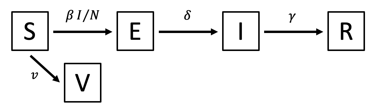
- Extend the SEIR model to include a vaccinated class:
- Draw the model diagram. Answer: See above.
- Implement the model in R starting from your SEIR code. Answer: See example solution.
Practical 2: Advanced use of deSolve
Solutions for practical 2 are found below.
Return to the practical here.