Estimating the overdispersion in COVID-19 transmission using outbreak sizes outside China
Aim
To estimate the level of overdispersion in COVID-19 transmission from the worldwide case count data.
Methods summary
- We extracted the number of imported/local cases in the affected countries from the WHO situation report 38 published on 27 February 2020.
- Assuming that the offspring distribution (distribution of the number of secondary transmissions) for COVID-19 cases is an identically- and independently-distributed negative-binomial distribution, we estimated the parameters of the negative-binomial distribution (reproduction number R0 and overdispersion k using the likelihood of observing the reported number of imported/local cases (outbreak size) of COVID-19 for each country.
- The outbreak size may grow in countries with an ongoing outbreak; using the current outbreak size as the final size for such countries may introduce bias. We assumed that the growth of a cluster in a country had not been ceased if the latest reported cases were within 7 days before 27 February 2020, and adjusted the likelihood for these countries by using the condition that the final cluster size has to be at least as large as the currently observed number of cases.
Key findings
- The offspring distribution of COVID-19 is highly overdispersed.
- For the likely range of R0 of 2-3, the overdispersion parameter k was estimated to be around 0.1, suggesting that the majority of secondary transmission is caused by a very small fraction of individuals (80% of transmissions caused by ~10% of the total cases).
- Joint estimation of R0 and k indicated it is likely that R0 > 1.4 and k < 0.2. The current data and model did not provide evidence on the upper bound of R0.
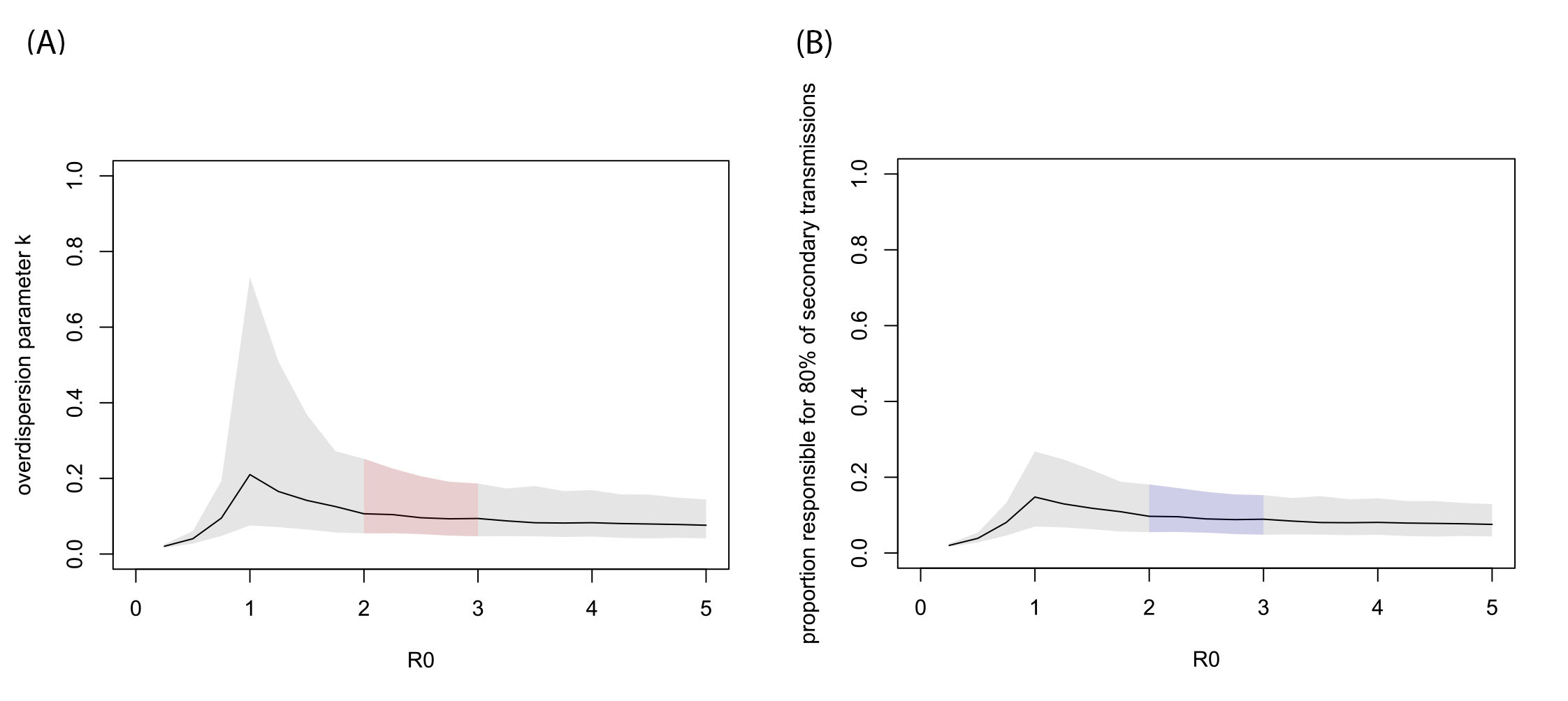
Figure 1. MCMC estimates given assumed R0 values. (A) Estimated overestimation parameter for various basic reproduction number R0. (B) Proportion of infected individuals responsible for 80% of the total secondary transmissions (p80%). The black lines show the median estimates given fixed R0 values and the grey shaded areas indicate 95% CrIs. The regions corresponding to the likely range of R0 (2-3) are indicated by colour.
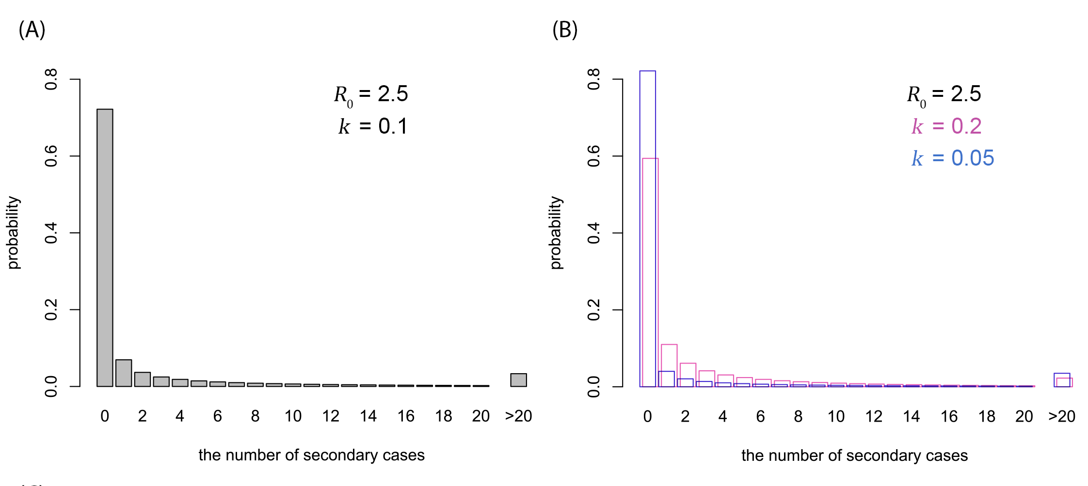
Figure 2. Possible offspring distributions of COVID-19. (A) Offspring distribution corresponding to R0 = 2.5 and k = 0.1 (median estimate). (B) Offspring distribution corresponding to R0 = 2.5 and k = 0.05 (95% CrI lower bound), 0.2 (upper bound). The probability mass functions of negative-binomial distributions are shown.
Table 1. Credible intervals from a joint estimation
| Parameter | Prior distribution | 95% lower bound | 95% upper bound |
|---|---|---|---|
| \(R_0\) | \(\mathcal N(\mu=3,\sigma=5)\) | 1.4 | 11.6 |
| \(k\) | \(\mathrm{HalfNormal}(\sigma=10)\) for the reciprocal \(k^{-1}\) | 0.04 | 0.2 |
Limitations
- We used the confirmed case counts reported to WHO and did not account for possible underreporting of cases.
- Reported cases whose site of infection classified as unknown, which should in principle be counted as either imported or local cases, were excluded from analysis.
- The distinction between countries with and without ongoing outbreak (7 days without any new confirmation of cases) was arbitrary and the results may be sensitive to this assumption.
Detailed methods
Full details and the underlying scripts can be found on a Github page.
Data source
We extracted the number of imported/local cases in the affected countries from the WHO situation report 38 published on 27 February 2020, which, at the time of writing, is the latest report of the number of imported/local cases in each country (from the situation report 40, WHO no longer reports the number of cases stratified by the site of infection). We defined imported cases as the cases whose likely site of infection is outside the reporting country, and the local cases as those whose likely site of infection is inside the reporting country. Those whose site of infection under investigation were excluded from the analysis. In Egypt and Iran, no imported cases have been confirmed which cause the likelihood value to be zero. Data in these two countries were excluded.
To distinguish between countries with and without an ongoing outbreak, we extracted daily case counts from an online resource (COVID2019.app) and determined the dates of the latest case confirmation for each country (as of 27 February).
Final outbreak size
Assume that the offspring distribution for COVID-19 cases is an i.i.d. negative-binomial distribution. The probability mass function for the final cluster size resulting from s initial cases is, according to Blumberg et al., given by
\[ c(x;s)=P(X=x;s)=\frac{ks}{kx+x-s}\binom{kx+x-s}{x-s}\frac{\left(\frac{R_0} k\right)^{x-s}}{\left(1+\frac{R_0} k\right)^{kx+x-s}}. \]
If the observed case counts are part of an ongoing outbreak in a country, cluster sizes may grow in the future. To address this issue, we adjusted the likelihood corresponding those countries with ongoing outbreak by only using the condition that the final cluster size of such a country has to be larger than the currently observed number of cases. The corresponding likelihood function is
\[ c_\mathrm{o}(x;s)=P(X\geq x;s)=1-\sum_{m=0}^{x}c(m;s)+c(x;s) \]
Defining countries with ongoing outbreak and total likelihood
\[ L(R_0,k)=\prod_{i\in A}P(X=x_i;s_i)\prod_{i\in B}P(X\geq x_i;s_i) \]
Estimating overdispersion parameter
Proportion responsible for 80% of transmissions
Following Grantz et al., we calculated the estimated proportion of infected individuals responsible for 80% of secondary transmissions caused. Such proportion p80% is given as
\[ 1-p_{80\%}=\int_0^{X}\mathrm{NB}\left(\lfloor x\rfloor;k,\frac{k}{R_0+k}\right)dx, \]
where (X) satisfies
\[ 1-0.8=\frac 1{R_0}\int_0^{X}\lfloor x\rfloor\mathrm{NB}\left(\lfloor x\rfloor;k,\frac{k}{R_0+k}\right)dx. \]
Note that
\[ \frac 1{R_0}\int_0^{X}\lfloor x\rfloor\mathrm{NB}\left(\lfloor x\rfloor;k,\frac{k}{R_0+k}\right)dx=\int_0^{X-1}\mathrm{NB}\left(\lfloor x\rfloor;k+1,\frac{k}{R_0+k}\right)dx. \]
We computed p80% for each MCMC sample to yield median and 95% CrIs.